The sf package
The sf (simple features) package can read and save shapefiles, and it plays nicely with the dpylr functions you’ve been learning. Let’s install it.
install.packages("sf")To load a shapefile, use the function st_read(). The st stands for spatial and temporal data.
DOWNLOAD — Census shapefile
- Download the ZIP file above for an example shapefile.
- Move the file to your project’s data folder.
- Unzip the file
Read the data using st_read("shapefile file location")
library(dplyr)
library(sf)
census <- st_read("data/Census2010_med_household_income.shp", stringsAsFactors = F)When you view the data you will see all the attributes of the shapefile stored in the first columns, and the spatial information stored in a final column named geometry.
# View your new spatial data table
glimpse(census)## Observations: 436
## Variables: 18
## $ OBJECTID <dbl> 1, 2, 3, 4, 5, 6, 7, 8, 9, 10, 11, 12, 13, 14, 15, ...
## $ NAME10 <chr> "120.01", "121.01", "121.02", "223.01", "261.01", "...
## $ INTPTLAT10 <chr> "+44.8970126", "+44.8953840", "+44.8980613", "+44.9...
## $ INTPTLON10 <chr> "-093.3054316", "-093.2360565", "-093.2152830", "-0...
## $ GEOID101 <dbl> 27053012001, 27053012101, 27053012102, 27053022301,...
## $ GEOID <chr> "1400000US27053012001", "1400000US27053012101", "14...
## $ GEOID2 <dbl> 27053012001, 27053012101, 27053012102, 27053022301,...
## $ AssocDegre <dbl> 52.2, 27.7, 28.7, 54.1, 50.9, 32.7, 48.7, 29.5, 58....
## $ Bachelor_A <dbl> 8.3, 14.6, 8.5, 30.3, 9.7, 21.8, 24.6, 0.0, 15.3, 1...
## $ Total_HHol <dbl> 2631, 1359, 1306, 1048, 1273, 1400, 1183, 1100, 117...
## $ Recvd_Fsta <dbl> 37, 254, 106, 15, 18, 74, 0, 4, 35, 175, 256, 131, ...
## $ Total_HH_1 <dbl> 2631, 1359, 1306, 1048, 1273, 1400, 1183, 1100, 117...
## $ HHold_MedI <dbl> 78060, 31612, 54183, 71250, 77145, 66341, 108150, 1...
## $ NoHigherEd <dbl> 21.0, 65.7, 32.1, 19.4, 21.9, 18.0, 21.6, 43.3, 34....
## $ TotalPopCo <dbl> 5922, 3405, 2648, 2113, 3206, 2776, 3219, 2824, 298...
## $ NoCollegeD <dbl> 0.3546099, 1.9295154, 1.2122356, 0.9181259, 0.68309...
## $ SNAP_Recvd <dbl> 0.6247889, 7.4596182, 4.0030211, 0.7098912, 0.56144...
## $ geometry <MULTIPOLYGON [m]> MULTIPOLYGON (((-10387144 5..., MULTIP...Try plot(census) to see an overview of all the shapefile’s attributes.
Quick plots
Plot all variables
# Colors each polygon by attribute
census %>% plot(max.plot = 9)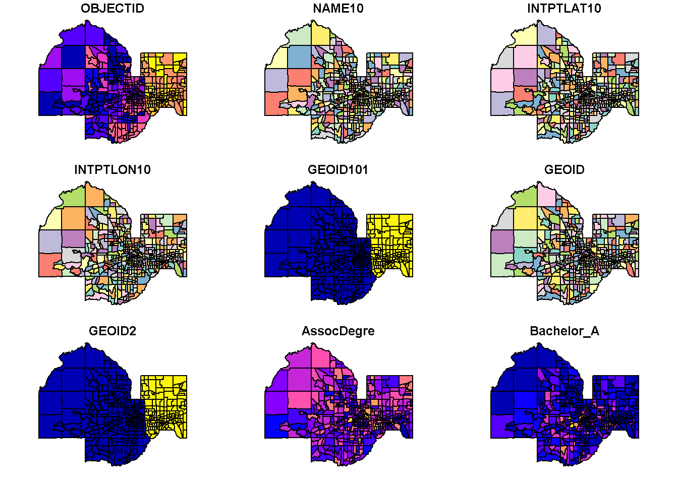
Plot a single variable
# Use select() to pick a single attribute
census %>% select(HHold_MedI) %>% plot()
Add grid lines
# Add graticules
census %>% select(HHold_MedI) %>% plot(graticule = T, axes = T)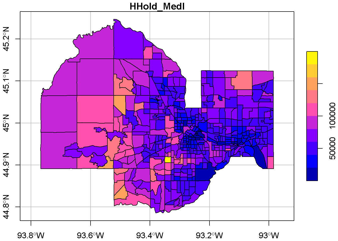
Plot with ggplot2 and viridis colors.
Run the code below to get the latest development version of ggplot2 and the viridis color palette.
install.packages("devtools")
devtools::install_github("tidyverse/ggplot2")
install.packages("viridis")Now you’re ready to make some ggplot maps.
# Load updated ggplot2 and colors
library(ggplot2)
library(viridis)
ggplot(census) +
geom_sf(aes(fill = HHold_MedI)) +
scale_fill_viridis() +
labs(title = "Median Household Income by Census tract")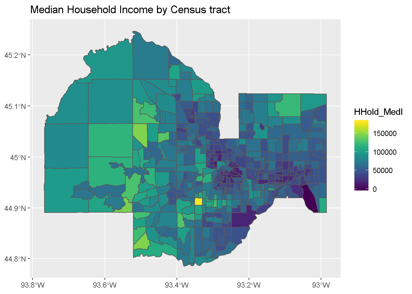
Transform coordinates
Current coordinate reference system (CRS)
census %>% st_crs()## Coordinate Reference System:
## EPSG: 3857
## proj4string: "+proj=merc +a=6378137 +b=6378137 +lat_ts=0.0 +lon_0=0.0 +x_0=0.0 +y_0=0 +k=1.0 +units=m +nadgrids=@null +wktext +no_defs"EPSG number for lat/long web coordinates - 4326
Web maps like Google and OpenStreets use the spherical Mercator projected coordinate system: EPSG#: 3857.
(See https://epsg.io/3857)
However, the coordinates shown to the user are primarily in : EPSG#: 4326.
(See https://epsg.io/4326)
To make Anne Morris’ day, ask her a question about coordinate reference systems.
EPSG number for UTM coordinates: 26915
Minnesota tends to use UTM coordinates for official business. They look like really big numbers, kind of like this: 475340, 5010480. They’re easy to put in the wrong order, so it helps to remember that the latitude (or Y-direction or N-S direction) is the one with an extra digit.
UTM coordinates are broken up into different zones to help reduce the errors of mapping a sphere to a flat surface. Minnesota uses UTM zone 15N. If you’re serious about maps, you should go ahead and get this tatooed to your right shoulder.
The EPSG code for UTM zone 15N is 26915.
(See https://epsg.io/26915)
Warning: When you save UTM coordinates in Excel or R, it’s best to switch the columns to text. It will save you from finding all of your coordinates being rounded by an overly helpful computer.
Create a new map in UTM coordinates
# Transform coordinates
census_utm <- census %>% st_transform(26915)
# Quick plot
census_utm %>% select(HHold_MedI) %>% plot()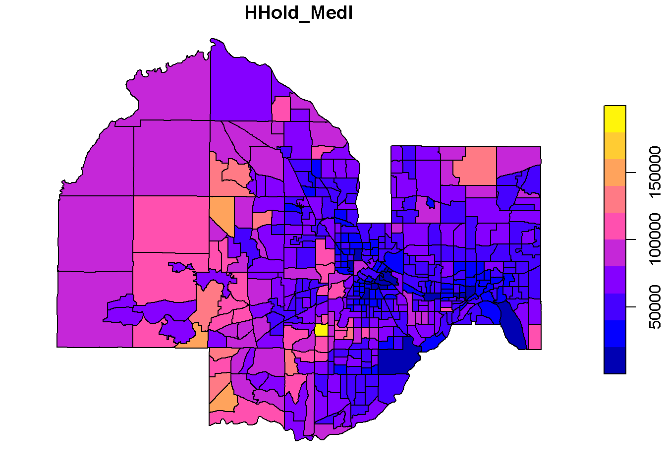
Wow! Can you see the difference?
Centroids
# Calculate Census tract centroids
tract_centers <- census_utm %>% st_centroid()
# Quick plot
tract_centers %>% plot()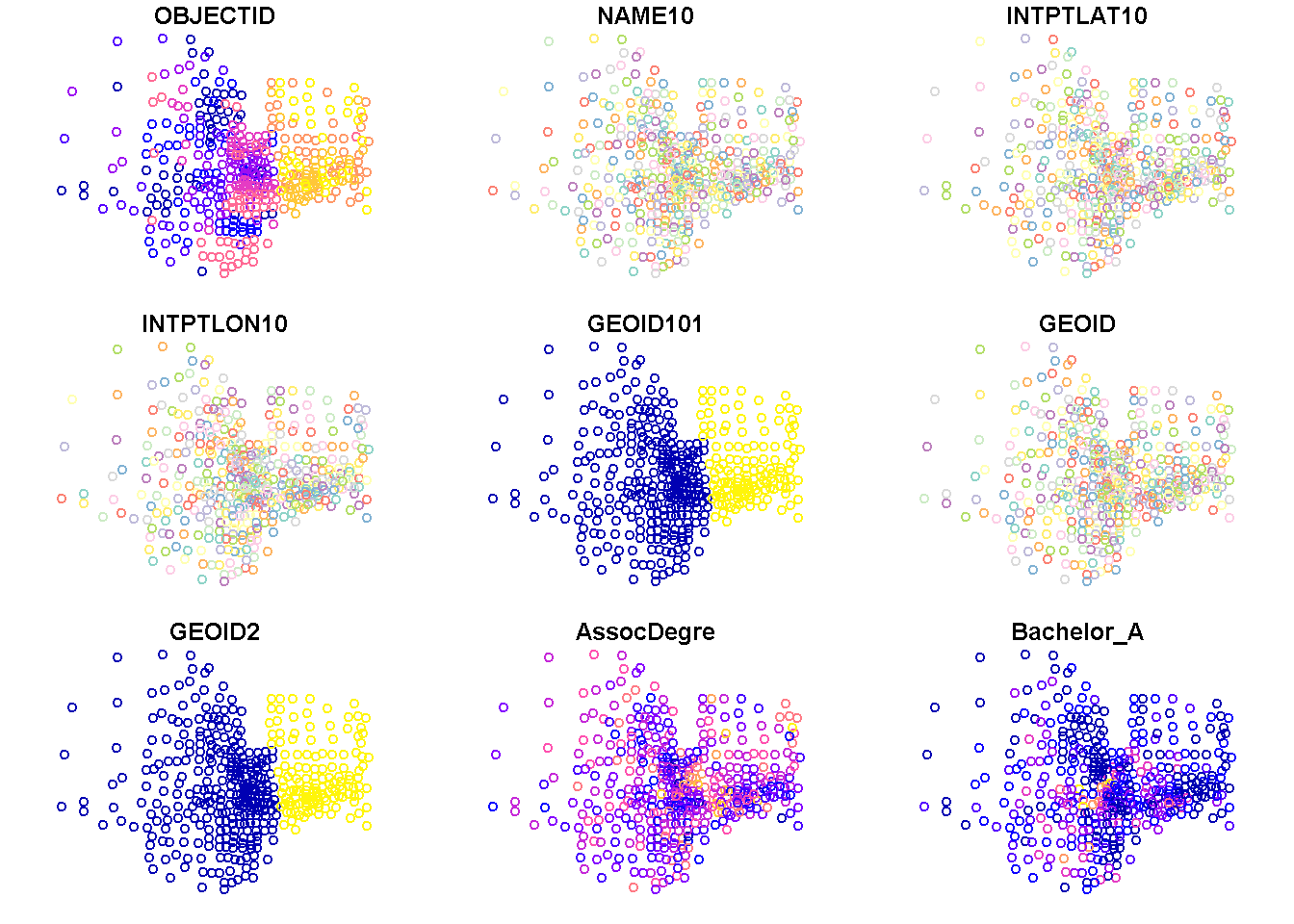
Add UTM centroid coordinates as new data columns
# Get centroid coordinates
center_coords <- st_coordinates(tract_centers) %>% as_data_frame()
# Add centroid coordinates as columns to polygon data
census_utm <- census_utm %>%
mutate(utm_x = center_coords$X,
utm_y = center_coords$Y)
# Check if it worked
names(census_utm)## [1] "OBJECTID" "NAME10" "INTPTLAT10" "INTPTLON10" "GEOID101"
## [6] "GEOID" "GEOID2" "AssocDegre" "Bachelor_A" "Total_HHol"
## [11] "Recvd_Fsta" "Total_HH_1" "HHold_MedI" "NoHigherEd" "TotalPopCo"
## [16] "NoCollegeD" "SNAP_Recvd" "geometry" "utm_x" "utm_y"glimpse(census_utm)## Observations: 436
## Variables: 20
## $ OBJECTID <dbl> 1, 2, 3, 4, 5, 6, 7, 8, 9, 10, 11, 12, 13, 14, 15, ...
## $ NAME10 <chr> "120.01", "121.01", "121.02", "223.01", "261.01", "...
## $ INTPTLAT10 <chr> "+44.8970126", "+44.8953840", "+44.8980613", "+44.9...
## $ INTPTLON10 <chr> "-093.3054316", "-093.2360565", "-093.2152830", "-0...
## $ GEOID101 <dbl> 27053012001, 27053012101, 27053012102, 27053022301,...
## $ GEOID <chr> "1400000US27053012001", "1400000US27053012101", "14...
## $ GEOID2 <dbl> 27053012001, 27053012101, 27053012102, 27053022301,...
## $ AssocDegre <dbl> 52.2, 27.7, 28.7, 54.1, 50.9, 32.7, 48.7, 29.5, 58....
## $ Bachelor_A <dbl> 8.3, 14.6, 8.5, 30.3, 9.7, 21.8, 24.6, 0.0, 15.3, 1...
## $ Total_HHol <dbl> 2631, 1359, 1306, 1048, 1273, 1400, 1183, 1100, 117...
## $ Recvd_Fsta <dbl> 37, 254, 106, 15, 18, 74, 0, 4, 35, 175, 256, 131, ...
## $ Total_HH_1 <dbl> 2631, 1359, 1306, 1048, 1273, 1400, 1183, 1100, 117...
## $ HHold_MedI <dbl> 78060, 31612, 54183, 71250, 77145, 66341, 108150, 1...
## $ NoHigherEd <dbl> 21.0, 65.7, 32.1, 19.4, 21.9, 18.0, 21.6, 43.3, 34....
## $ TotalPopCo <dbl> 5922, 3405, 2648, 2113, 3206, 2776, 3219, 2824, 298...
## $ NoCollegeD <dbl> 0.3546099, 1.9295154, 1.2122356, 0.9181259, 0.68309...
## $ SNAP_Recvd <dbl> 0.6247889, 7.4596182, 4.0030211, 0.7098912, 0.56144...
## $ geometry <MULTIPOLYGON [m]> MULTIPOLYGON (((475580.9 49..., MULTIP...
## $ utm_x <dbl> 475925.2, 481549.1, 483002.3, 468882.9, 465465.5, 4...
## $ utm_y <dbl> 4971482, 4971497, 4971649, 4976925, 4975884, 498025...Area calculations with st_area()
# Add area column for each Census tracts
census_utm <- census_utm %>% mutate(area = st_area(geometry))
# Quick plot of BIGGEST 3 tracts
census_utm %>%
filter(rank(area) > 433) %>%
select(HHold_MedI) %>%
plot()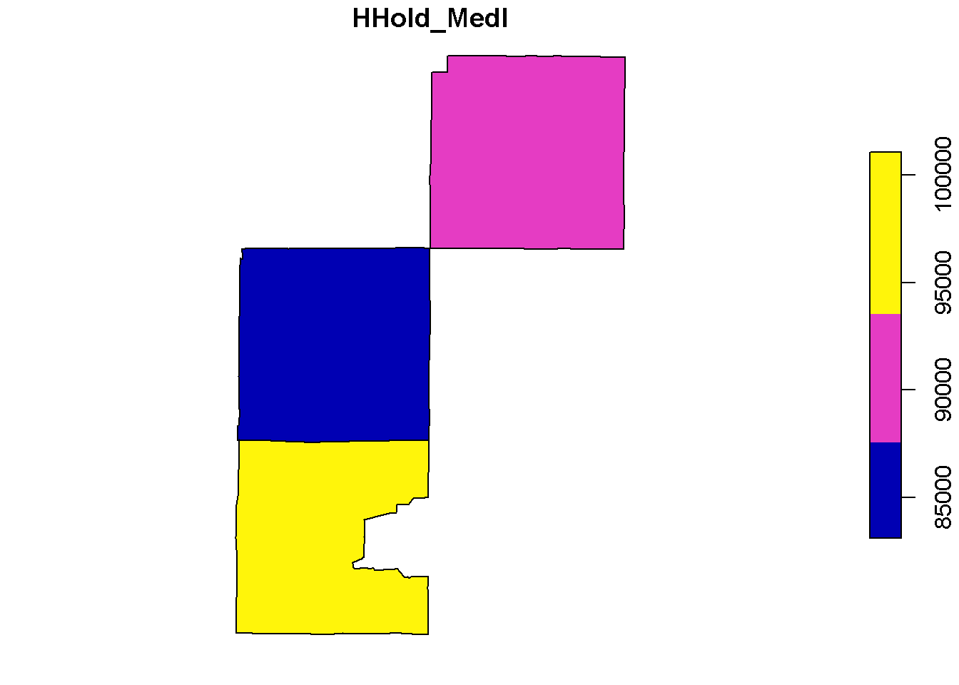
# Filter to top 3
big_tracts <- filter(census_utm, rank(area) > 433)
# Convert to a normal plain data_frame
big_tracts <- as_data_frame(big_tracts)
# Put a big dots to the 3 largest Census tracts
ggplot(census_utm) +
geom_sf(aes(fill = HHold_MedI)) +
geom_point(data = big_tracts, aes(x = utm_x, y = utm_y), size = 7) +
scale_fill_viridis() +
labs(title = "Median Household Income by Census tract")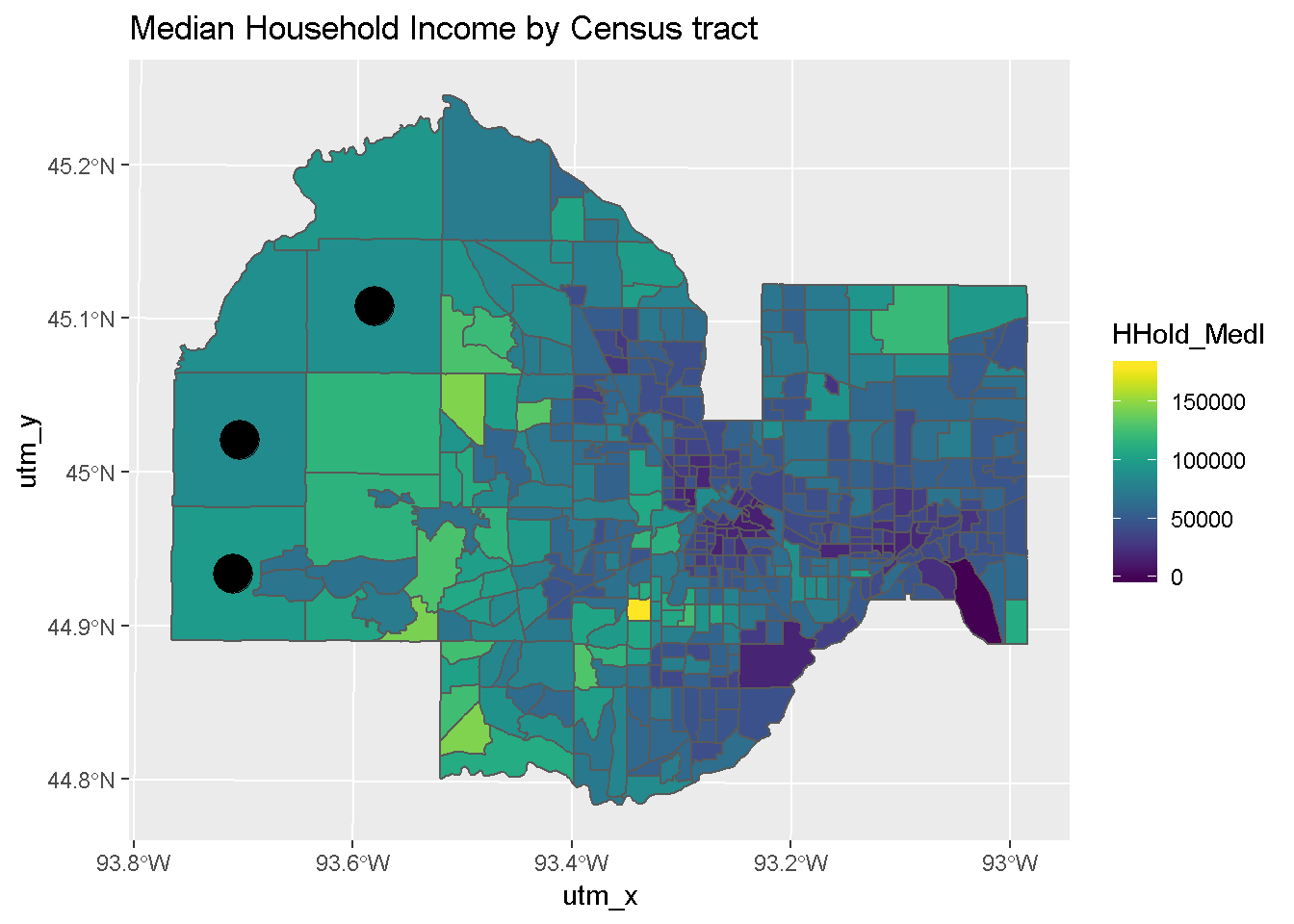
Interactive map with leaflet
Install the leaflet package to make quick interactive maps.
install.packages("leaflet")
A map you can zoom and click on!
library(leaflet)
# Leaflet uses coordinates in the normal lat/long Google map flavor.
# EPSG
census <- st_transform(census, 4326)
# Check coordinate system
# You want "+datum=WGS84"
st_crs(census)## Coordinate Reference System:
## EPSG: 4326
## proj4string: "+proj=longlat +datum=WGS84 +no_defs"# Create a color legend based on HHold_MedI
legend_colors <- colorQuantile("Blues", census$HHold_MedI, n = 7)
# Polygon map colored by HHold_MedI
web_map <- leaflet(census) %>%
addProviderTiles(providers$OpenStreetMap) %>%
addPolygons(fillColor = ~legend_colors(HHold_MedI),
fillOpacity = 0.75,
color = "white", # Border color
weight = 1, # Border width
popup = paste("Census Tract: ", census$GEOID,
"<br> Median HH Income: ", census$HHold_MedI))
# Show map
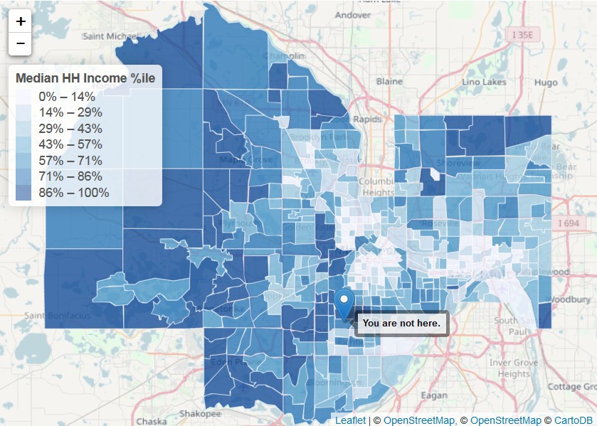
web_map# Click on it.Let’s make the background gray, and add special marker and a legend.
# Add gray base map and a marker for your favorite Tract
web_map <- web_map %>%
addProviderTiles(providers$CartoDB.Positron, options = providerTileOptions(opacity = 0.5)) %>%
addMarkers(lng = census$INTPTLON10[1] %>% as.numeric(),
lat = census$INTPTLAT10[1] %>% as.numeric(),
label = "You are not here.",
labelOptions = labelOptions(noHide = T),
popup = paste("These people make more $ than you."))
# Add a floating legend
web_map <- web_map %>%
addLegend("topleft",
pal = legend_colors,
values = ~HHold_MedI,
title = "Median HH Income %ile")
# Reprint map
web_mapDistance calculations with st_distance()
# Find distance between the center of first 3 Census tracts
distances <- census_utm[1:3, ] %>% st_distance()
census_utm[1:3, ] %>% select("HHold_MedI") %>% plot(pch = 19)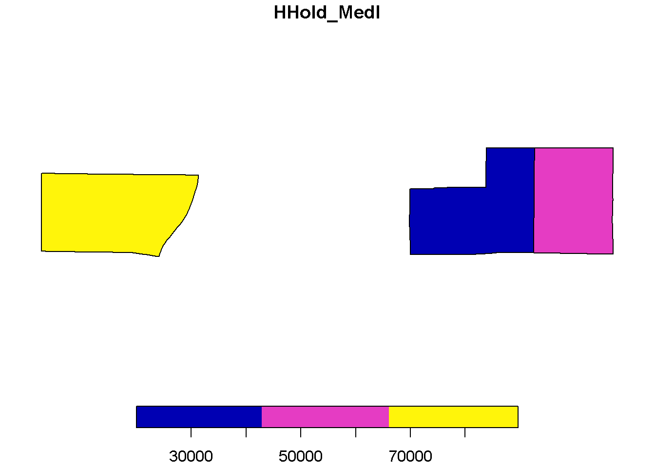
# Using the centroids we calculated earlier,
## Find distance between the center of first census tract and all other census tracts
distances <- tract_centers %>% st_distance()
# Add all distances to the polygon dataframe
census_utm <- census_utm %>% mutate(distance = distances[1, ])
# Take a look
## Apparently it is a total distance of 0 meters away from itself.
glimpse(census_utm)## Observations: 436
## Variables: 22
## $ OBJECTID <dbl> 1, 2, 3, 4, 5, 6, 7, 8, 9, 10, 11, 12, 13, 14, 15, ...
## $ NAME10 <chr> "120.01", "121.01", "121.02", "223.01", "261.01", "...
## $ INTPTLAT10 <chr> "+44.8970126", "+44.8953840", "+44.8980613", "+44.9...
## $ INTPTLON10 <chr> "-093.3054316", "-093.2360565", "-093.2152830", "-0...
## $ GEOID101 <dbl> 27053012001, 27053012101, 27053012102, 27053022301,...
## $ GEOID <chr> "1400000US27053012001", "1400000US27053012101", "14...
## $ GEOID2 <dbl> 27053012001, 27053012101, 27053012102, 27053022301,...
## $ AssocDegre <dbl> 52.2, 27.7, 28.7, 54.1, 50.9, 32.7, 48.7, 29.5, 58....
## $ Bachelor_A <dbl> 8.3, 14.6, 8.5, 30.3, 9.7, 21.8, 24.6, 0.0, 15.3, 1...
## $ Total_HHol <dbl> 2631, 1359, 1306, 1048, 1273, 1400, 1183, 1100, 117...
## $ Recvd_Fsta <dbl> 37, 254, 106, 15, 18, 74, 0, 4, 35, 175, 256, 131, ...
## $ Total_HH_1 <dbl> 2631, 1359, 1306, 1048, 1273, 1400, 1183, 1100, 117...
## $ HHold_MedI <dbl> 78060, 31612, 54183, 71250, 77145, 66341, 108150, 1...
## $ NoHigherEd <dbl> 21.0, 65.7, 32.1, 19.4, 21.9, 18.0, 21.6, 43.3, 34....
## $ TotalPopCo <dbl> 5922, 3405, 2648, 2113, 3206, 2776, 3219, 2824, 298...
## $ NoCollegeD <dbl> 0.3546099, 1.9295154, 1.2122356, 0.9181259, 0.68309...
## $ SNAP_Recvd <dbl> 0.6247889, 7.4596182, 4.0030211, 0.7098912, 0.56144...
## $ geometry <MULTIPOLYGON [m]> MULTIPOLYGON (((475580.9 49..., MULTIP...
## $ utm_x <dbl> 475925.2, 481549.1, 483002.3, 468882.9, 465465.5, 4...
## $ utm_y <dbl> 4971482, 4971497, 4971649, 4976925, 4975884, 498025...
## $ area [m^2] 2625248 [m^2], 2388985 [m^2], 1964491 [m^2], 152147...
## $ distance [m] 0.000 [m], 5623.902 [m], 7079.086 [m], 8900.067 [m], ...Download Census data
The tigris package is great for Census boundary files, and the tidycensus provides access to all of the updated ACS demographic data. With their powers combined you can make all the maps.
Spatial polygons
Let’s install the tigris package.
install.packages(tigris)
Minnesota tracts
library(tigris)
# Load geography
mn_tracts <- tracts(state = "MN", cb = TRUE)
# Plot map
plot(mn_tracts)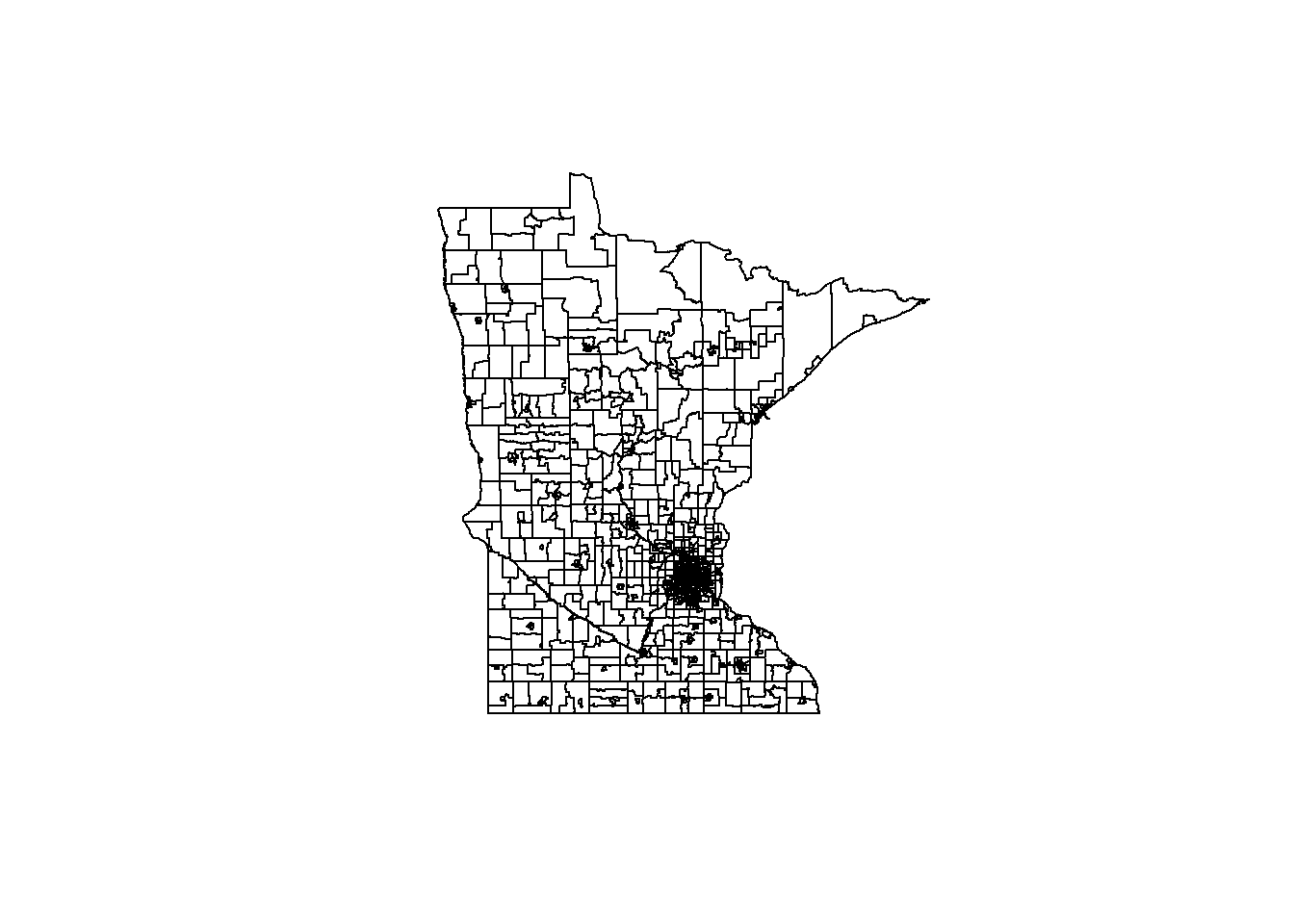
Midwest Counties
# Load geography
midw_counties <- counties(state = c("MN","SD","ND", "WI"), cb = TRUE)
plot(midw_counties, col = midw_counties$STATEFP, stroke = "white")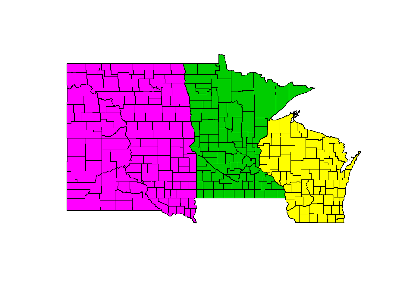
Tribal block groups
# Load geography
tribal_bgs <- tribal_block_groups()
# Convert to sf filetype
tribal_bgs <- st_as_sf(tribal_bgs)# Interactive leaflet map
trib_map <- leaflet(tribal_bgs) %>%
addProviderTiles("CartoDB.Positron") %>%
addPolygons(fillColor = "steelblue",
color = "black",
weight = 0.5,
opacity = 0.75,
popup = ~GEOID)
trib_map