
Good morning!


We like R.
We aren’t computer scientists and that’s okay!
We make lots of mistakes. Mistakes are funny. You can laugh with us.
1 What’s R?
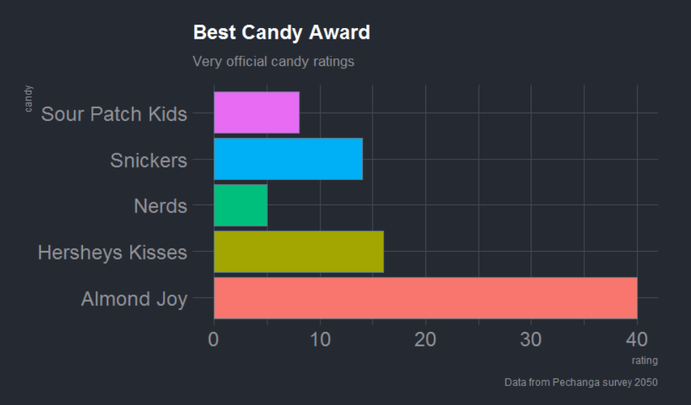
Let’s launch ourselves into the unknown and make a candy plot. With a little copy-pasting we can make an informative chart of everyone’s favorite candy.
Since you have the best taste, let’s make your candy BIG .
Instructions
- Copy all the code below. Hold SHIFT and highlight all of the lines, until you reach
theme_ft_rc(base_size = 14).
#-----------  Install packages  ---------------#
install.packages("ggplot2")
install.packages("readr")
install.packages("hrbrthemes")


#-------------  Load packages  ----------------#
library(ggplot2)
library(readr)
library(hrbrthemes)


#---------------- Candy data ------------------#
survey <- read_csv('candy,rating
                   "Snickers",        14
                   "Almond Joy",      40
                   "Hersheys Kisses", 16
                   "Nerds",           5
                   "Sour Patch Kids", 8')


#------- Column plot with dark theme ---------#
ggplot(survey,
       aes(x = candy, y = rating)) +
  geom_col(aes(fill = candy), show.legend = FALSE) +
  labs(title    = "Candy Champions",
       subtitle = "Very official candy ratings",
       caption  = "Data from Pechanga survey 2050") +
  coord_flip() +
  #scale_fill_viridis_d()
theme_ft_rc(base_size = 14) - Open R Studio
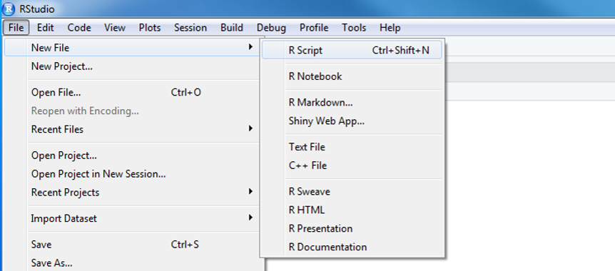
- Select File > New File > R Script. You will see a code editor window open.
- Or click the paper icon with the green plus at the top left.
- Paste the copied code into the upper left hand window. This is your code editor.
- Highlight all of the code and hit CTRL+ENTER.
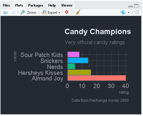
This chart should appear in the lower right of RStudio.
- Change the name of a candy to something even better.
- Re-run the code again.
- Try increasing the number next to the new candy.
Bonus
- Add another candy and rating to the data.
- Add your name to the subtitle.
- Delete the hashtag in front of the
scale_viridis...line.
- What happens when you re-run the code?
- Change the
show.legend =value toTRUE
- What happens?
Congrats rebel droid!
Spock-tip!
- You don’t need to memorize everything. Yay!
- Absorb what’s possible. You can always look up details later.
- R is a tool. You can use it without understanding all the inner workings.
- You are free to break things. Create errors. Make the computer angry. Learn through “mistakes”. R will forgive you.
- Cheat if you’re stuck.
- There’s no test and you can’t really win. So share with your neighbors. Copy others.
Introductions
Let’s introduce ourselves and the data we love. Chat with your partner and get to know 3 things about them.
Things to share:
- Your name or Star Wars alias
- Types of data you have
- Who you share it with
- Something you want to get from the workshop
- The funniest part of your data
- The most repetitive part? Hint: Maybe this is something you can automate with R
Go Team
We’re going to need to work together to help Rey get off the dusty planet Jakku. Use each other as a resource. Share ideas, share code, collaborate. Make bad jokes.
Here’s one:
Which Jedi is best at opening PDF files? >
A: Adobe Wan Kenobi?

2 RStudio - A Grand Tour
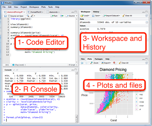
1. Code Editor
This is where you write your scripts and document your work. Move your cursor to a line of code and then click [Ctrl] + [Enter] to run the code. The tabs at the top of the code editor show the scripts and data sets you have open. The script is your home and where we spend most of our time.
3. Workspace
This pane shows all of the objects and functions that you have created, as well as a history of the code you have run during your current session. The environment tab shows all of your objects and functions. The history tab shows the code you have run. Note the broom icon below the Connections tab. This cleans shop and allows you to clear all of the objects in your workspace.
2. R Console
This is where code is actually executed by the computer. It shows code that you have run and the messages returned by that code. You can input code directly into the console and run it, but it won’t be saved for later. That’s why we usually run our code directly from a script in the code editor.
You may see some scary warnings and errors appear here after running code. Warnings are helpful messages that let you know the results may not be exactly what you expected. Errors on the other hand, mean the code was unable to run. Usually this means there was a typo, or we forgot to run an important step higher up in our script.
4. Plots and files
These tabs allow you to view and open files in your current directory, view plots and other visual objects like maps, view your installed packages and their functions, and access the help window.
The Files tab is especially handy for finding a file you want and clicking it to op_en it. You can also click the More option and select “Show Folder in a New Window” as a shortcut to open your project folder.
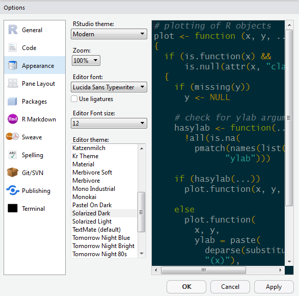
Customize R Studio
Let’s add a little style so R Studio feels like home. Follow these steps to change the font-size and color scheme:
- Go to Tools on the top navigation bar.
- Choose
Global Options... - Choose
Appearancewith the paint bucket. - Increase the
Editor Font size - Pick an Editor theme you like.
- The default is
Textmateif you want to go back
- The default is
Why R?
R Community
- See the R Community page.
- MPCA sharing + questions - R questions
- Finding R Help - Get Help!
- R Cheatsheets
When we use R
- To connect to databases
- To read data from websites
- To document and share methods
- When data will have frequent updates
- When we want to improve a process over time
R is for reading
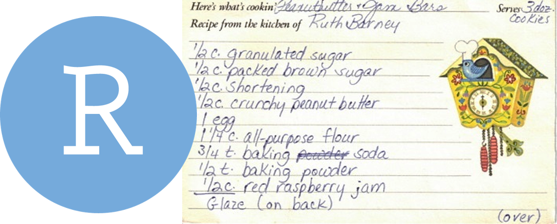
Lucky for us, R code doesn’t have to be only math equations. R let’s us do data analysis in a step-by-step fashion, much like creating a recipe for cookies. And just like a recipe, we can start at the top and read our way down to the bottom.
Example ozone analysis
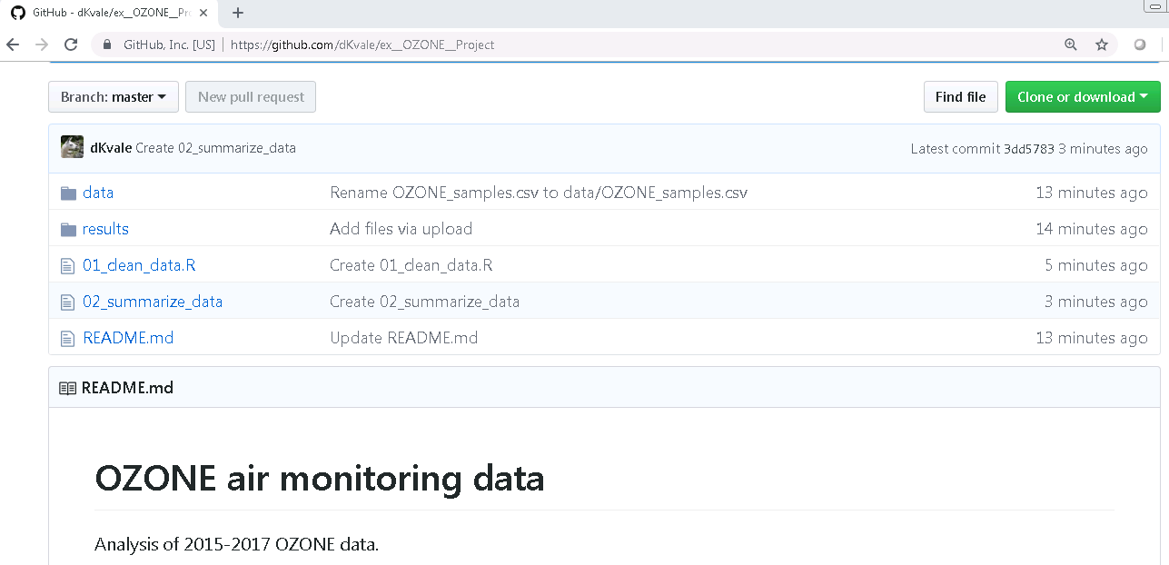
Here’s an example air monitoring project from start to finish.
EXAMPLE - Ozone data project >
Imagine we just received 3 years worth of ozone monitoring data to summarize. Fun! Below is an example workflow we might follow using R.
- Read the data
- Simplify columns
- Plot the data
- Clean the data
- View the data closer
- Summarize the data
- Save the results
- Share with friends
0. Start a new project
We’ll name this project: "2019_Ozone"
1. Read the data
library(readr)

# Read a file from the web
air_data <- read_csv("https://itep-r.netlify.com/data/OZONE_samples_demo.csv")| SITE | Date | OZONE | TEMP_F |
|---|---|---|---|
| 27-137-7001 | 2018-05-16 | 9 | 53.6 |
| 27-137-7001 | 2016-10-01 | 7 | 51.8 |
| 27-137-7554 | 2017-09-30 | 7 | 48.2 |
| 27-137-7554 | 2017-05-01 | 3 | 44.6 |
| 27-137-7554 | 2016-06-02 | 15 | 74.6 |
2. Simplify column names
library(janitor)

# Capital letters and spaces make things more difficult
# Let's clean them out
air_data <- clean_names(air_data)
3. Plot the data
library(ggplot2)

ggplot(air_data, aes(x = temp_f, y = ozone)) +
    geom_point(alpha = 0.2) +
    geom_smooth(method = "lm")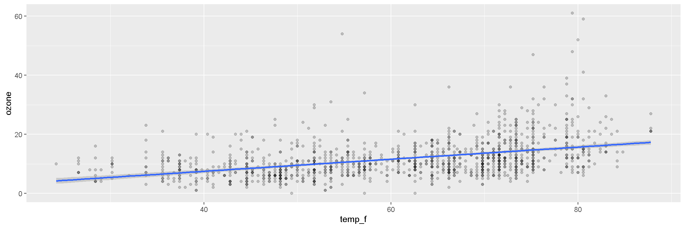
4. Clean the data
library(dplyr)

# Drop values out of range
air_data <- air_data %>% filter(ozone > 0, temp_f < 199)

# Convert all samples to PPB
air_data <- air_data %>%
            mutate(OZONE = ifelse(units == "PPM", ozone * 1000,
                                  ozone))
5. View the data closer
ggplot(air_data, aes(x = temp_f, y = ozone)) +
    geom_point(alpha = 0.2, size = 3) +
    geom_smooth(method = "lm") +
    facet_wrap(~site) +
    labs(title = "Ozone increases with temperature",
         subtitle = "Observations from 2015-2017")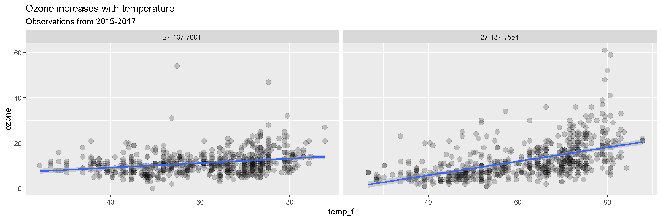
6. Summarize the data
air_data <- air_data %>%
            group_by(site, year) %>%
            summarize(avg_ozone = mean(ozone) %>% round(2),
avg_temp = mean(temp_f) %>% round(2))| site | year | avg_ozone | avg_temp |
|---|---|---|---|
| 27-137-7001 | 2016 | 11.01 | 60.74 |
| 27-137-7001 | 2017 | 11.26 | 60.66 |
| 27-137-7001 | 2018 | 11.54 | 60.59 |
| 27-137-7554 | 2016 | 12.23 | 61.23 |
| 27-137-7554 | 2017 | 11.81 | 60.98 |
| 27-137-7554 | 2018 | 12.87 | 61.02 |
7. Save the results
Save the final data table
air_data %>% write_csv("results/2015-17_ozone_summary.csv")Save the site plot to PDF
ggsave("results/2015-2017 - Ozone vs Temp.pdf")8. Share with friends
Having an exact record of what you did can be great documentation for yourself and others. It’s also handy when you want to repeat the same analysis on new data. Then you only need to copy the script, update the read data line, and push run to get a whole new set of fancy charts.
3 Show & Tell
Insert magic here…
Data awaits us…

Let’s go find some trouble. While BB8 works on tracking down data for us from his droid friends, we’ll get to know his internal computer.
New data -> New R project
Let’s make a new project for our Jakku scrap analysis.
Step 1: Start a new project
- In Rstudio select File from the top menu bar
- Choose New Project…
- Choose New Directory
- Choose New Project
- Enter a project name such as
"starwars" - Select Browse… and choose a folder where you normally perform your work.
- Click Create Project
Step 2: Open a new script
- File > New File > R Script
- Click the floppy disk save icon
- Give it a name:
jakku1.Rorday1.Rwill work well
4 Names and things
You can assign values to new objects using the “left arrow” <-. It’s typed with a less-than sign < followed by a hyphen -. It’s more officially known as the assignment operator.
Let’s make a droid!
Try adding the code below to your R script to create an object called droid.
Assignment operator
# Create a new object
droid <- "bb7"

droid

# Give it a new value
droid <- "bb8"

droid
To run a line of code in your script, click the cursor anywhere on that line and press CTRL+ENTER.
The droid wants a friend. Let’s create a Wookie named Chewbacca.
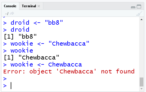
wookie <- "Chewbacca"

wookie
Break some things
# To save text to an object we use quotes: "text"

# Try this:
wookie <- Chewbacca
Error!
Without quotes, R looks for an object called Chewbacca, and then lets you know that it couldn’t find one. Let’s try again after adding quotation marks around Chewbacca.
Colors decoded
Blue shows the exact code you ran.
Black is the result of the code. A [1] in front means there is one item in that object, and its value is bb8.
Red shows Errors & Warnings. Warnings are ok, they inform you that the result may not be exactly what you expect.
Copy objects
# To copy an object, assign it to a new name
wookie2 <- wookie


# Or overwrite an object with new "text"
wookie <- "Tarfful"

wookie


# Wookie2 stays the same
wookie2
Numbers!
wookie_salary <- 500

# Let's give Chewbacca a big raise $$$
wookie_salary <- 500 * 2

# Print new salary
wookie_salary

# We can also use the object to multiply
wookie_salary * 2

# To save the change we assign it back to itself
wookie_salary <- wookie_salary * 2
Drop and remove data
You can drop objects with the remove function rm(). Try it out on some of your wookies.
# Delete objects to clean-up your Environment
rm(wookie)

rm(wookie2)
Explore!
How can we get the wookie object back?
Hint: You are allowed to re-run your code. You can even highlight everything and re-run ALL of the code.
Deleting data is okay! >
Don’t worry about deleting data or objects in R. You can always recreate them! When R loads your data it copies the contents and then cuts off any connection to the original data. So your original data remain safe and won’t suffer any accidental changes. That means if something disappears or goes wrong in R, it’s okay. We can re-run the R script to get the data back.
It’s common to frequently re-run your entire R script during your analysis.4.1 What’s a good name?
Everything has a name in R and you can name things almost anything you like, even TOP_SECRET_shhhhhh... or data_McData_face.
Sadly, there are a few restrictions. R doesn’t like names to include spaces or special characters found in math equations, like +, -, *, \, /, =, !, or ).
Explore!
Try running some of these examples. Find new ways to create errors. The more broken the better! Half of learning R is finding what doesn’t work.
# What happens when you add these to your R script?
n wookies <- 5

n*wookies <- 5

n_wookies <- 5

n.wookies <- 5

wookies! <- "Everyone"
Names with numbers
# Names cannot begin with a number
1st_wookie <- "Chewbacca"

88b <- "droid"

# But they can contain numbers
wookie1    <- "Chewbacca"

bb8 <- "droid"

# What if you have 10,000 wookies?
n_wookies <- 10,000  # Error

n_wookies <- 10000
4.2 Collect multiple items
We can put multiple values inside c() to make a vector of items. It’s like a chain of items, where each additional item is connected by a comma. The c stands for concatenate or to collect.
Let’s use c() to create a few vectors of names.
# Create a character vector and name it starwars_characters
starwars_characters <- c("Luke", "Leia", "Han Solo")

# Print starwars_characters
starwars_characters
## [1] "Luke" "Leia" "Han Solo"# Create a numeric vector and name it starwars_ages
starwars_ages <- c(19,19,25)
# Print the ages to the console
starwars_ages## [1] 19 19 25Note
Take a look at the new additions to your Environment pane located on the top right.
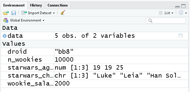
This window shows all of the objects we’ve created so far and the types of data they contain. It’s a great first look to see if our script ran successfully. You can click the broom icon to sweep everything out and start with a clean slate.
4.3 Make a table
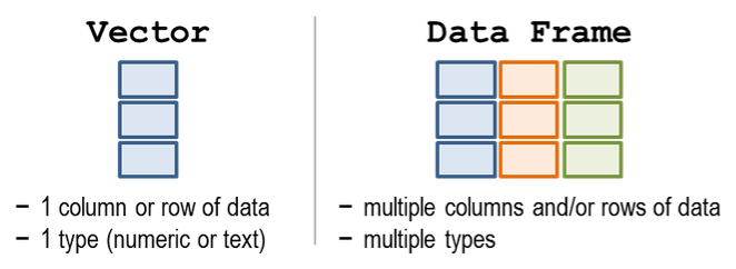
A table in R is known as a data frame. We can think of it as a group of columns, where each column is made from a vector. Data frames in R have columns of data that are all the same length.
Let’s make a data frame with two columns to hold the character names and their ages.
# Create table with 2 columns: characters & ages
starwars_df <- data.frame(characters = starwars_characters,
                          ages       = starwars_ages)

# Print the starwars_df data frame to the console
starwars_df
## characters ages
## 1 Luke 19
## 2 Leia 19
## 3 Han Solo 25Explore!
Add a 3rd column that lists their fathers names:
c("Darth", "Darth", "Unknown")
starwars_df <- data.frame(characters  = starwars_characters,
                          ages        = starwars_ages,
                          fathers     = __________________)
starwars_df <- data.frame(characters  = starwars_characters,
                          ages        = starwars_ages,
                          fathers     = c("Darth", "Darth", "Unknown"))
Show all values in $column_name
Use the $ sign after the name of your table to see the values in one of your columns.
# View the "ages" column in starwars_df
starwars_df$ages
## [1] 19 19 25Pop Quiz!
Which of these object names are valid? (Hint: You can test them.)
my starwars fandom
my_wookies55
5wookies
my-wookie
Wookies!!!
Show solution
my_wookies55
Yes!! The FORCE is strong with you!
4.4 Add a #comment
The lines of code in the scripts that start with a # in front are called comments. Every line that starts with a # is ignored and won’t be run as R code. You can use the # to add notes in your script to make it easier for others and yourself to understand what is happening and why. You can also use comments to add warnings or instructions for others using your code.
5 Read data
The first step of a good scrap audit is reading in some data to figure out where all the scrap is coming from. Here’s a small dataset showing the scrap economy on Jakku. It was salvaged from a crash site, but the transfer was incomplete.
| origin | destination | item | amount | price_d |
|---|---|---|---|---|
| Outskirts | Raiders | Bulkhead | 332 | 300 |
| Niima Outpost | Trade caravan | Hull panels | 1120 | 286 |
| Cratertown | Plutt | Hyperdrives | 45 | 45 |
| Tro—- | Ta—- | So—* | 1 | 10—- |
This looks like it could be useful. Now, if only we had some more data to work with…
New Message (1)
Incoming… BB8
BB8: Beep boop Beep.
BB8: I intercepted a large scrapper data set from droid 4P-L of Junk Boss Plutt.
Receiving data now…
scrap_records.csv
item,origin,destination,amount,units,price_per_pound
Flight recorder,Outskirts,Niima Outpost,887,Tons,590.93
Proximity sensor,Outskirts,Raiders,7081,Tons,1229.03
Aural sensor,Tuanul,Raiders,707,Tons,145.27
Electromagnetic filter,Tuanul,Niima Outpost,107,Tons,188.2
...
You: Yikes! This looks like a mess! What can I do with this?
CSV to the rescue
The main data format used in R is the CSV (comma-separated values). A CSV is a simple text file that can be opened in R and most other stats software, including Excel. It looks squished together as plain text, but that’s okay! When opened in R, the text becomes a familiar looking table with columns and rows.
Before we launch ahead, let’s add a package to R that will help us read CSV files.
How to save a CSV from Excel
Step 1: Open your Excel file.
Step 2: Save as CSV
- Go to File
- Save As
- Browse to your project folder
- Save as type: _CSV (Comma Delimited) (*.csv)_
- Any of the CSV options will work
- Any of the CSV options will work
- Click Yes
- Close Excel (Click “Don’t Save” as much as you need to. Seriously, we just saved it. Why won’t Excel just leave us alone?)
Step 3: Return to RStudio and open your project. Look at your Files tab in the lower right window. Click on the CSV file you saved and choose View File.
Success!
6 Add packages 📦 (R Apps)
What is an R package?
A package is a small add-on for R, it’s like a phone App for your phone. They add capabilities like statistical functions, mapping powers, and special charts to R. In order to use a new package we first need to install it. Let’s try it!

The readr package helps import data into R in different formats. It helps you out by cleaning the data of extra white space and formatting tricky date formats automatically.
Add a package to your library
- Open RStudio
- Type
install.packages("readr")in the lower left console - Press Enter
- Wait two seconds
- Open the
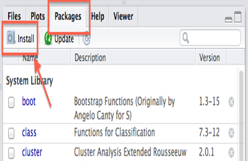
Packagestab in the lower right window of RStudio to see the packages in your library- Use the search bar to find the
readrpackage
- Use the search bar to find the
Your installed packages are stored in your R library. The Packages tab on the right shows all of the available packages installed in your library. When you want to use one of them, you load it in R.
Loading a package is like opening an App on your phone. To load a package we use the library() function. Once you load it, the package will stay loaded until you close RStudio.
Note
The 2 steps to using a packag in R:
install.packages("package-name")library(package-name)
6.1 Read the data
Let’s load the readr package so we can use the read_csv() function to read the Jakku scrap data.
#install.packages("readr")
library(readr)

read_csv("https://itep-r.netlify.com/data/starwars_scrap_jakku.csv")
## # A tibble: 1,132 x 7
## receipt_date item origin destination amount units price_per_pound
## <chr> <chr> <chr> <chr> <dbl> <chr> <dbl>
## 1 4/1/2013 Flight re~ Outski~ Niima Outp~ 887 Tons 591.
## 2 4/2/2013 Proximity~ Outski~ Raiders 7081 Tons 1229.
## 3 4/3/2013 Vitus-Ser~ Reestki Raiders 4901 Tons 226.
## 4 4/4/2013 Aural sen~ Tuanul Raiders 707 Tons 145.
## 5 4/5/2013 Electroma~ Tuanul Niima Outp~ 107 Tons 188.
## 6 4/6/2013 Proximity~ Tuanul Trade cara~ 32109 Tons 1229.
## 7 4/7/2013 Hyperdriv~ Tuanul Trade cara~ 862 Tons 1485.
## 8 4/8/2013 Landing j~ Reestki Niima Outp~ 13944 Tons 1497.
## 9 4/9/2013 Electroma~ Crater~ Raiders 7788 Tons 188.
## 10 4/10/2013 Sublight ~ Outski~ Niima Outp~ 10642 Tons 7211.
## # ... with 1,122 more rowsName the data
Where did the data go after you read it into R? When we want to work with the data in R, we need to give it a name with the assignment operator: <-.
# Read in scrap data and set name to "scrap"
scrap <- read_csv("https://itep-r.netlify.com/data/starwars_scrap_jakku.csv")

# Type the name of the table to view it in the console
scrap
## # A tibble: 1,132 x 7
## receipt_date item origin destination amount units price_per_pound
## <chr> <chr> <chr> <chr> <dbl> <chr> <dbl>
## 1 4/1/2013 Flight re~ Outski~ Niima Outp~ 887 Tons 591.
## 2 4/2/2013 Proximity~ Outski~ Raiders 7081 Tons 1229.
## 3 4/3/2013 Vitus-Ser~ Reestki Raiders 4901 Tons 226.
## 4 4/4/2013 Aural sen~ Tuanul Raiders 707 Tons 145.
## 5 4/5/2013 Electroma~ Tuanul Niima Outp~ 107 Tons 188.
## 6 4/6/2013 Proximity~ Tuanul Trade cara~ 32109 Tons 1229.
## 7 4/7/2013 Hyperdriv~ Tuanul Trade cara~ 862 Tons 1485.
## 8 4/8/2013 Landing j~ Reestki Niima Outp~ 13944 Tons 1497.
## 9 4/9/2013 Electroma~ Crater~ Raiders 7788 Tons 188.
## 10 4/10/2013 Sublight ~ Outski~ Niima Outp~ 10642 Tons 7211.
## # ... with 1,122 more rowsSpock-tip!
Notice the row of <three> letter abbreviations under the column names? These describe the data type of each column.
<chr>stands for character vector or a string of characters. Examples: “apple”, “apple5”, “5 red apples”
<int>stands for integer. Examples: 5, 34, 1071
<dbl>stands for double. Examples: 5.0000, 3.4E-6, 10.7106
We’ll explore more data types later on, such as dates and logical (TRUE/FALSE).
Pop Quiz!
1. What data type is the destination column?
letters
character
TRUE/FALSE
numbers
Show solution
character
Woop! You got this.
2. What package does read_csv() come from?
dinosaur
get_data
readr
dplyr
Show solution
readr
Great job! You are Jedi worthy!
3. How would you load the package junkfinder?
junkfinder()
library(junkfinder)
load(junkfinder)
gogo_gadget(junkfinder)
Show solution
library("junkfinder")
Excellent! Keep the streak going.
BONUS Function options
Function options
Functions have options that you can change to control their behavior. You can set these optins using arguments. Let’s look at a few of the arguments for the function read_csv().
Skip a row
Sometimes you may want to ignore the first row in your data file, especially an EPA file that includes a disclaimer on the first row. Yes EPA, we’re looking at you. Please stop.
Let’s open the help window with ?read_csv and try to find an argument that can help us.
?read_csvThere’s a lot of them! But the skip argument looks like it could be helpful. Take a look at the description near the bottom. The default is skip = 0, which reads every line, but we can skip the first line by writing skip = 1. Let’s try.
read_csv("https://itep-r.netlify.com/data/starwars_scrap_jakku.csv", skip = 1)Limit the number of rows
Other types of data have weird last rows that are a subtotal or just report “END OF DATA”. Sometimes we want read_csv to ignore the last row, or only pull in a million lines because you don’t want to bog down the memory on an old laptop.
Let’s look through the help window to find an argument that can help us. Type ?read_csv and scroll down.
The n_max argument looks like it could be helpful. The default is n_max = Inf, which means it will read every line, but we can limit the lines we read to only one hundred by using n_max = 100.
# Read in 100 rows
small_data <- read_csv("https://itep-r.netlify.com/data/starwars_scrap_jakku.csv", skip = 1, n_max = 100)

# Remove the data
rm(small_data)
Spock-tip!
To see all of a function’s arguments:
- Enter its name in the console followed by a parenthesis.
- Type
read_csv(
- Type
- Press
TABon the keyboard. - Explore the drop-down menu of the available arguments.
Pop Quiz!
Which of these is a valid function call?
train(“concentrate” “Force”)
shoot, “lightsaber”, “Death Ray”
replicate(100000000, “clones”)
fight(until Empire conquered)
scrap(100 Datapads, “Hyperdrives”)
Show solution
replicate(100000000, "clones")
Correct! You are ready to audit a Junk dealer.
7 ggplot2
Plot the data, Plot the data, Plot the data
In data analysis it’s super important to look at your data early and often. For that we use a new package called ggplot2!
Install it by running the following in your Console:
install.packages("ggplot2")
Note
You can also install packages from the Packages tab in the lower right window of RStudio.
A column plot
Here’s a simple chart showing the total amount of scrap sold from each origin location.
library(ggplot2)ggplot(scrap, aes(y = amount, x = origin)) +
geom_col() +
labs(title = "Which origin sold the most scrap?") +
theme_gray()## Warning: Removed 910 rows containing missing values (position_stack).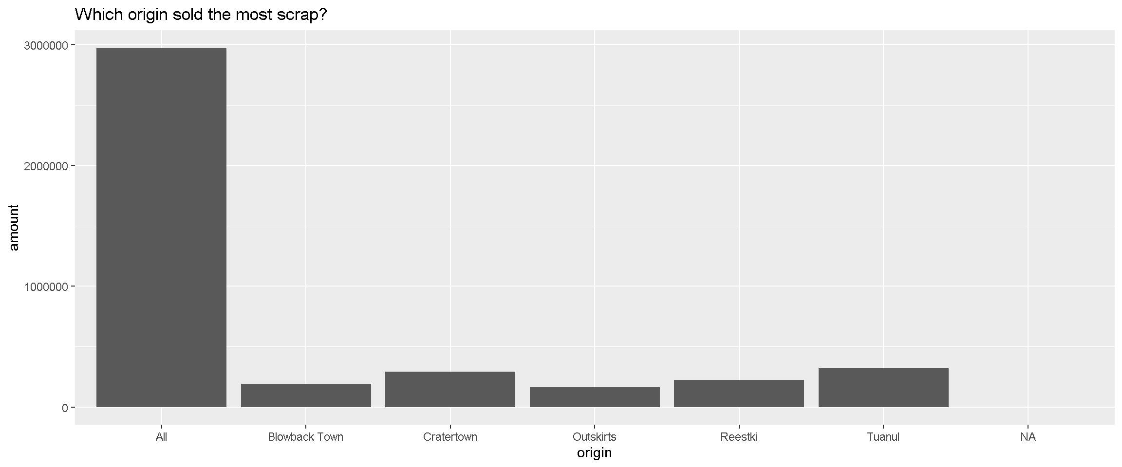
Well, well, well, it looks like there is an All category we should look into more. Either there is a town hogging all the scrap or the data needs some cleaning.
Explore!
Try changing theme_gray() to theme_dark(). What changes on the chart? What stays the same?
Try another theme: theme_classic() or theme_void() or delete the entire line and the + above to see what the default settings are.
You can view all available theme options at ggplot2 themes.
BONUS Does the order of arguments matter?
Let’s say you had a function called feed_porgs(), which has 3 arguments:
feed_porgs(breakfast = "fish", lunch = "veggies", dinner = "clams").
A shorthand to write this would be:
feed_porgs("fish", "veggies", "clams").
This works out just fine because all of the arguments were entered in the default order, the same as above.
What happens if we write:
feed_porgs("veggies", "clams", "fish")
Now the function sends veggies to the porgs for breakfast because that is the first argument.
Unfortunately, that’s no good for the porgs. So if we really want to write “veggies” first, we’ll need to tell R which food item belongs to which meal.
Like this:
feed_porgs(lunch = "veggies", breakfast = "fish", dinner = "clams").
What about read_csv()?
For read_csv we wrote:
read_csv(scrap_file, column_names, skip = 1)
R assumes that the first argument (the data file) is scrap_file and that the 2nd argument “col_names” should be set to column_names. Next, the skip = argument is included explicitly because skip is the 10th argument in read_csv().
If we don’t include skip=, R will assume the value 1 is meant for the function’s 3rd argument.
Get help!
Lost in an ERROR message? Is something behaving strangely and want to know why? Want ideas for a new chart?
Go to Help! for troubleshooting, cheatsheets, and other learning resources.
Robot recap
What packages have we added to our
library?What new functions have we learned?
Key terms
package |
An add-on for R that contains new functions that someone created to help you. It’s like an App for R. | |
library |
The name of the folder that stores all your packages, and the function used to load a package. | |
function |
Functions perform an operation on your data and returns a result. The function sum() takes a series of values and returns the sum for you. |
|
argument |
Arguments are options or inputs that you pass to a function to change how it behaves. The argument skip = 1 tells the read_csv() function to ignore the first row when reading in a data file. To see the default values for a function you can type ?read_csv in the console. |