1 dplyr
2 glimpse() & summary()
Your analysis toolbox
3 Porg tables
4 select()
5 Sort with arrange()
R BINGO!
6 filter()
7 mutate()
8 Save our data
9 Plots with ggplot2
10 Shutdown complete
New data -> New project!

Data exploration

1 dplyr

You’ve unlocked a new package!

dplyr is the go-to tool for exploring, re-arranging, and summarizing data.

Use install.packages("dplyr") to add dplyr to your library.

Then try loading the package from your library to test if it was installed.

library(dplyr)

Get to know your data frame

Use these functions to describe your data.

Data frame info

Function		Information
`names(scrap)`		column names
`nrow(...)`		number of rows
`ncol(...)`		number of columns
`summary(...)`		summary of all column values (ex. max, mean, median)
`glimpse(...)`		column names + a glimpse of first values (requires dplyr package)

2 `glimpse()` & `summary()`

glimpse() tells you what type of data and how much data you have.

Let’s read the data into R and give these a whirl.

library(readr)
library(dplyr)

scrap <- read_csv("https://itep-r.netlify.com/data/starwars_scrap_jakku.csv")

# View your whole dataframe and the types of data it contains
glimpse(scrap)

## Observations: 1,132
## Variables: 7
## $ receipt_date    <chr> "4/1/2013", "4/2/2013", "4/3/2013", "4/4/2013"...
## $ item            <chr> "Flight recorder", "Proximity sensor", "Vitus-...
## $ origin          <chr> "Outskirts", "Outskirts", "Reestki", "Tuanul",...
## $ destination     <chr> "Niima Outpost", "Raiders", "Raiders", "Raider...
## $ amount          <dbl> 887, 7081, 4901, 707, 107, 32109, 862, 13944, ...
## $ units           <chr> "Tons", "Tons", "Tons", "Tons", "Tons", "Tons"...
## $ price_per_pound <dbl> 590.93, 1229.03, 225.54, 145.27, 188.28, 1229....

summary() gives you a quick report of your numeric data.

# Summary gives us the means, mins, and maxima 
summary(scrap)

##  receipt_date           item              origin         
##  Length:1132        Length:1132        Length:1132       
##  Class :character   Class :character   Class :character  
##  Mode  :character   Mode  :character   Mode  :character  
##                                                          
##                                                          
##                                                          
##                                                          
##  destination            amount           units          
##  Length:1132        Min.   :     65   Length:1132       
##  Class :character   1st Qu.:   1544   Class :character  
##  Mode  :character   Median :   4099   Mode  :character  
##                     Mean   :  18751                     
##                     3rd Qu.:   7475                     
##                     Max.   :2971601                     
##                     NA's   :910                         
##  price_per_pound   
##  Min.   :   145.3  
##  1st Qu.:   259.6  
##  Median :   790.7  
##  Mean   :  3811.7  
##  3rd Qu.:  1496.7  
##  Max.   :579215.3  
##  NA's   :910

Explore!

# Try some more on your own
nrow()

ncol()

names()

Your analysis toolbox

dplyr is the hero for most analysis tasks. With these six functions you can accomplish just about anything you want with your data.

Function Job

select() Select individual columns to drop or keep

arrange() Sort a table top-to-bottom based on the values of a column

filter() Keep only a subset of rows depending on the values of a column

mutate() Add new columns or update existing columns

summarize() Calculate a single summary for an entire table

group_by() Sort data into groups based on the values of a column

Function	Job
`select()`	Select individual columns to drop or keep
`arrange()`	Sort a table top-to-bottom based on the values of a column
`filter()`	Keep only a subset of rows depending on the values of a column
`mutate()`	Add new columns or update existing columns
`summarize()`	Calculate a single summary for an entire table
`group_by()`	Sort data into groups based on the values of a column

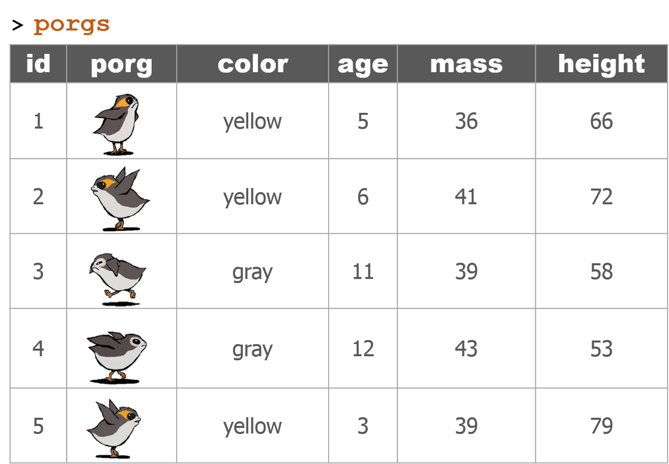
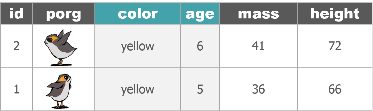
3 Porg tables

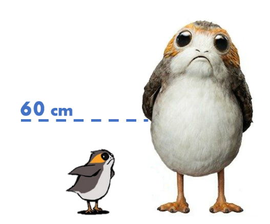
A poggle of porgs volunteered to help us demo the dplyr functions.

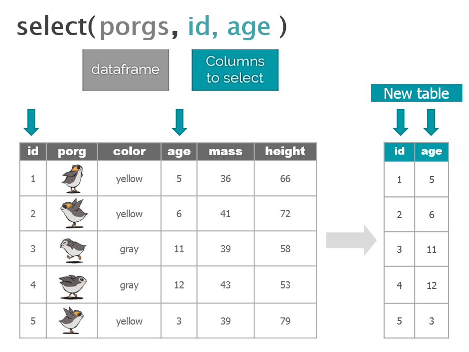
4 `select()`

Use the select() function to:

Drop columns you no longer need
Pull-out a few columns to create a new table
Rearrange or change the order of columns

Drop columns with a minus sign: `-col_name`

library(dplyr)
library(readr)

scrap <- read_csv("https://itep-r.netlify.com/data/starwars_scrap_jakku.csv")

# Drop the destination column
select(scrap, -destination)

## # A tibble: 1,132 x 6
##    receipt_date item                  origin   amount units price_per_pound
##    <chr>        <chr>                 <chr>     <dbl> <chr>           <dbl>
##  1 4/1/2013     Flight recorder       Outskir~    887 Tons             591.
##  2 4/2/2013     Proximity sensor      Outskir~   7081 Tons            1229.
##  3 4/3/2013     Vitus-Series Attitud~ Reestki    4901 Tons             226.
##  4 4/4/2013     Aural sensor          Tuanul      707 Tons             145.
##  5 4/5/2013     Electromagnetic disc~ Tuanul      107 Tons             188.
##  6 4/6/2013     Proximity sensor      Tuanul    32109 Tons            1229.
##  7 4/7/2013     Hyperdrive motivator  Tuanul      862 Tons            1485.
##  8 4/8/2013     Landing jet           Reestki   13944 Tons            1497.
##  9 4/9/2013     Electromagnetic disc~ Cratert~   7788 Tons             188.
## 10 4/10/2013    Sublight engine       Outskir~  10642 Tons            7211.
## # ... with 1,122 more rows

Drop multiple columns

Use -c(col_name1, col_name2) or -col_name1, -col_name2 to drop multiple columns.

# Drop the destination and units columns
select(scrap, -c(destination, units, amount))

## # A tibble: 1,132 x 4
##    receipt_date item                             origin     price_per_pound
##    <chr>        <chr>                            <chr>                <dbl>
##  1 4/1/2013     Flight recorder                  Outskirts             591.
##  2 4/2/2013     Proximity sensor                 Outskirts            1229.
##  3 4/3/2013     Vitus-Series Attitude Thrusters  Reestki               226.
##  4 4/4/2013     Aural sensor                     Tuanul                145.
##  5 4/5/2013     Electromagnetic discharge filter Tuanul                188.
##  6 4/6/2013     Proximity sensor                 Tuanul               1229.
##  7 4/7/2013     Hyperdrive motivator             Tuanul               1485.
##  8 4/8/2013     Landing jet                      Reestki              1497.
##  9 4/9/2013     Electromagnetic discharge filter Cratertown            188.
## 10 4/10/2013    Sublight engine                  Outskirts            7211.
## # ... with 1,122 more rows

Keep only 3 columns

# Keep item, amount and price_per_pound columns
select(scrap, item, amount, price_per_pound)

## # A tibble: 1,132 x 3
##    item                             amount price_per_pound
##    <chr>                             <dbl>           <dbl>
##  1 Flight recorder                     887            591.
##  2 Proximity sensor                   7081           1229.
##  3 Vitus-Series Attitude Thrusters    4901            226.
##  4 Aural sensor                        707            145.
##  5 Electromagnetic discharge filter    107            188.
##  6 Proximity sensor                  32109           1229.
##  7 Hyperdrive motivator                862           1485.
##  8 Landing jet                       13944           1497.
##  9 Electromagnetic discharge filter   7788            188.
## 10 Sublight engine                   10642           7211.
## # ... with 1,122 more rows

`everything()` else the same

select() also works to change the order of columns. The code below puts the item column first and then moves the units and amount columns directly after item.

We then keep evertyhing() else the same.

# Make the `item`, `units`, and `amount` columns the first three columns
# Leave `everything()` else in the same order
select(scrap, item, units, amount, everything())

## # A tibble: 1,132 x 7
##    item       units amount receipt_date origin  destination price_per_pound
##    <chr>      <chr>  <dbl> <chr>        <chr>   <chr>                 <dbl>
##  1 Flight re~ Tons     887 4/1/2013     Outski~ Niima Outp~            591.
##  2 Proximity~ Tons    7081 4/2/2013     Outski~ Raiders               1229.
##  3 Vitus-Ser~ Tons    4901 4/3/2013     Reestki Raiders                226.
##  4 Aural sen~ Tons     707 4/4/2013     Tuanul  Raiders                145.
##  5 Electroma~ Tons     107 4/5/2013     Tuanul  Niima Outp~            188.
##  6 Proximity~ Tons   32109 4/6/2013     Tuanul  Trade cara~           1229.
##  7 Hyperdriv~ Tons     862 4/7/2013     Tuanul  Trade cara~           1485.
##  8 Landing j~ Tons   13944 4/8/2013     Reestki Niima Outp~           1497.
##  9 Electroma~ Tons    7788 4/9/2013     Crater~ Raiders                188.
## 10 Sublight ~ Tons   10642 4/10/2013    Outski~ Niima Outp~           7211.
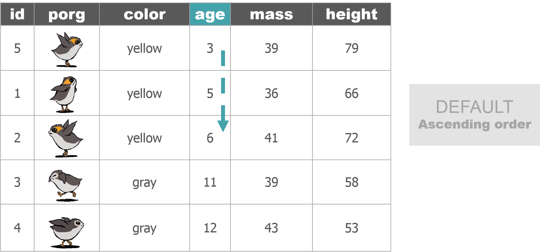
## # ... with 1,122 more rows

5 Sort with `arrange()`

Rey wants to know what the highest priced items are. Use arrange() to find the highest priced scrap item and see which origins might have a lot of them.

# Arrange scrap items by price
scrap <- arrange(scrap, price_per_pound)

# View the top 6 rows
head(scrap)

## # A tibble: 6 x 7
##   receipt_date item      origin    destination amount units price_per_pound
##   <chr>        <chr>     <chr>     <chr>        <dbl> <chr>           <dbl>
## 1 4/4/2013     Aural se~ Tuanul    Raiders        707 Tons             145.
## 2 5/22/2013    Aural se~ Outskirts Niima Outp~   3005 Tons             145.
## 3 5/23/2013    Aural se~ Tuanul    Raiders       6204 Tons             145.
## 4 6/4/2013     Aural se~ Tuanul    Raiders       3120 Tons             145.
## 5 6/10/2013    Aural se~ Blowback~ Niima Outp~   2312 Tons             145.
## 6 6/20/2013    Aural se~ Outskirts Trade cara~   6272 Tons             145.

What, only 145 credits!? That’s not much at all. Oh wait…that’s the smallest one on top.

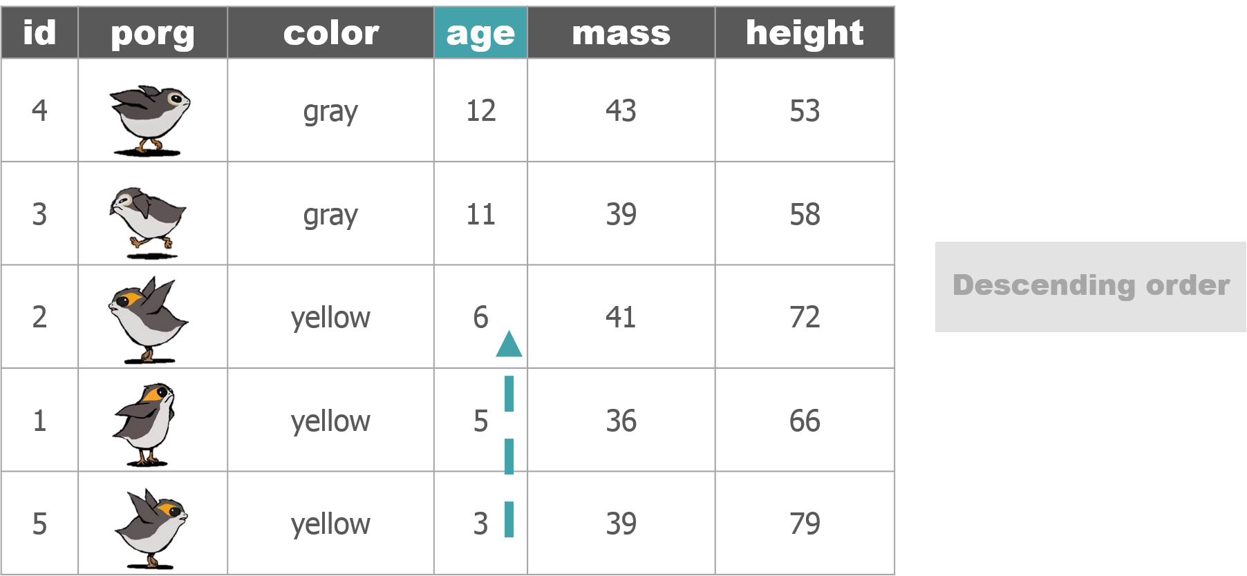
Big things first: `desc()`

To arrange a column in descending order with the biggest numbers on top, we use: desc(price_per_pound)

# Put most expensive items on top
scrap <- arrange(scrap, desc(price_per_pound))

# View the top 8 rows
head(scrap, 8)

## # A tibble: 8 x 7
##   receipt_date item      origin    destination amount units price_per_pound
##   <chr>        <chr>     <chr>     <chr>        <dbl> <chr>           <dbl>
## 1 12/31/2016   Total     All       All         2.97e6 Tons          579215.
## 2 4/10/2013    Sublight~ Outskirts Niima Outp~ 1.06e4 Tons            7211.
## 3 4/14/2013    Sublight~ Outskirts Raiders     2.38e3 Tons            7211.
## 4 4/15/2013    Sublight~ Craterto~ Raiders     6.31e3 Tons            7211.
## 5 4/16/2013    Sublight~ Tuanul    Trade cara~ 3.98e3 Tons            7211.
## 6 5/14/2013    Sublight~ Craterto~ Raiders     2.99e2 Tons            7211.
## 7 6/14/2013    Sublight~ Blowback~ Raiders     8.58e3 Tons            7211.
## 8 8/6/2013     Sublight~ Craterto~ Raiders     1.77e3 Tons            7211.

Explore!

Try arranging by more than one column, such as price_per_pound and amount. What happens?

Hint: You can view the entire table by clicking on it in the upper-right Environment tab.

Spock-tip!

When you save an arranged data table it maintains its order. This is perfect for sending people a quick Top 10 list of pollutants or sites.

R BINGO!

We don’t have free spaces. Sorry, we are very mean people.

We’re going to call-out the bingo words using an R function.

# Get pretty colors
install.packages("viridis")
library(viridis)
library(ggplot2)

# List of all the words
bingo_words <- c("median()", "nrow()", "glimpse()", "sum()", "head()", "tail()", "arrange()", "write_csv()", "geom_col()", "filter()", "ncol()", "sd()", "summarise()", "quantile()", "install.packages()", "geom_point()", "unique()", "select()", "mean()", "min()", "left_join()", "read_csv()", "nth()", "ggplot()", "library()", "n()")

# Shuffle the words randomly
bingo_words <- sample(bingo_words)

# Set the draw number
n <- 1

# Loop thru each word
for(n in 1:length(bingo_words)) {

  print(n)
  
  # Plot the word
  call_fun <- ggplot(data.frame(x = 1, y = 1), aes(x = 1, y = 1)) + 
        geom_point(color = sample(viridis_pal()(30), 1), size = 177) + 
        geom_label(label = bingo_words[n], size = 12) +
        labs(x = NULL, y = NULL) +
        theme_void()
  
  print(call_fun)
  
  readline(prompt="Press Enter...")
}

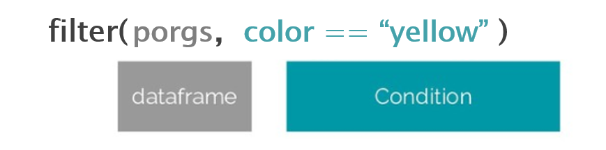
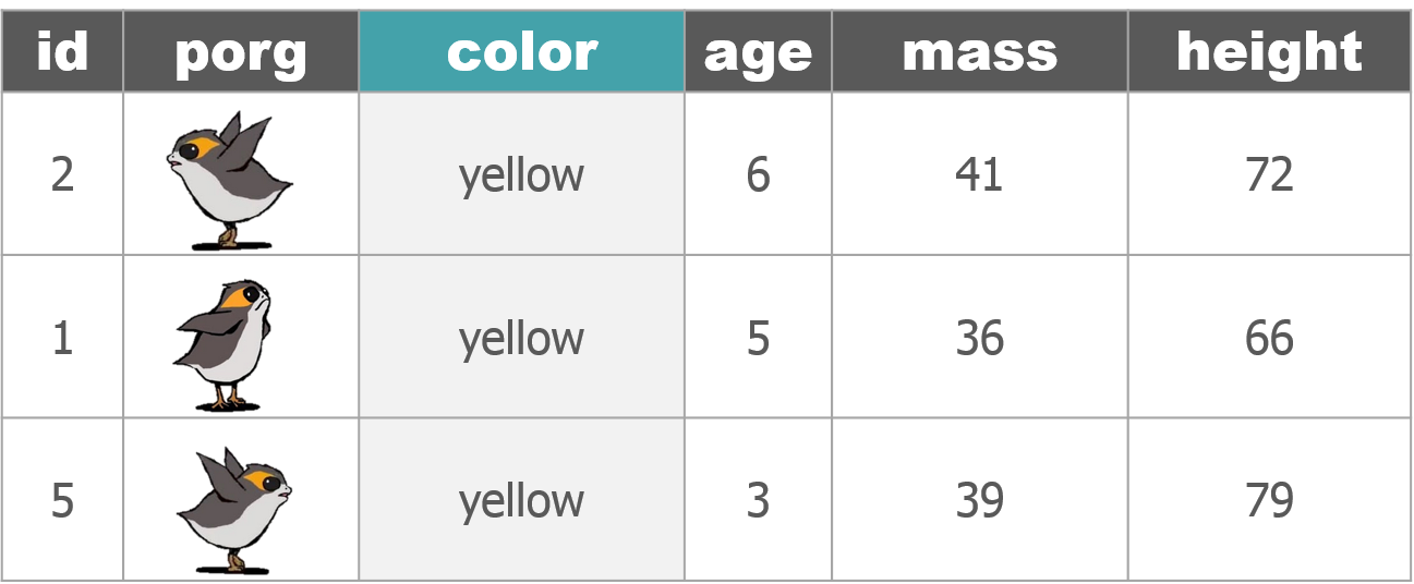
6 `filter()`

The filter() function creates a subset of the data based on the value of one or more columns. Let’s take a look at the records with the origin "All".

filter(scrap, origin == "All")

## # A tibble: 1 x 7
##   receipt_date item  origin destination  amount units price_per_pound
##   <chr>        <chr> <chr>  <chr>         <dbl> <chr>           <dbl>
## 1 12/31/2016   Total All    All         2971601 Tons          579215.

Spock-tip!

We use a == (double equals sign) for comparing values. A == makes the comparison “is it equal to?” and returns a True or False answer. So the code above will returns only the rows where the condition origin == "All" is TRUE.

A single equals sign = is used within functions to set options, for example read_csv(file = "starwars_scrap_jakku.csv"). It’s not a big deal if you mix them up the first time. R is often helpful and will let you know which one is needed.

Comparing values

We use a variety of comparisons when processing data. Sometimes we only want concentrations above a certain level, or days below a given temperature, or sites that have missing observations.

We use the Menu of comparisons below to find the data we want.

Menu of comparisons

Symbol Comparison

> greater than

>= greater than or equal to

< less than

<= less than or equal to

== equal to

!= NOT equal to

%in% value is in a list: X %in% c(1,3,7)

is.na(...) is the value missing?

str_detect(col_name, "word") “word” appears in text?

Symbol	Comparison
`>`	greater than
`>=`	greater than or equal to
`<`	less than
`<=`	less than or equal to
`==`	equal to
`!=`	NOT equal to
`%in%`	value is in a list: `X %in% c(1,3,7)`
`is.na(...)`	is the value missing?
`str_detect(col_name, "word")`	“word” appears in text?

Explore!

Try comparing some things in the console to see if you get what you’d expect. R doesn’t always think like we do.

4 != 5

4 == 4

4 < 3

4 > c(1, 3, 5)

5 == c(1, 3, 5)

5 %in% c(1, 3, 5)

2 %in% c(1, 3, 5)

2 == NA

6.1 Dropping rows

Let’s look at the data without the All category. Look in the comparison table above to find the NOT operator. We’re going to filter our data to keep only the origins that are NOT equal to “All”.

scrap <- filter(scrap, origin != "All")

We can arrange the data in ascending order by item to confirm the “All” category is gone.

# Arrange data
scrap <- arrange(scrap, item)

head(scrap)

## # A tibble: 6 x 7
##   receipt_date item      origin    destination amount units price_per_pound
##   <chr>        <chr>     <chr>     <chr>        <dbl> <chr>           <dbl>
## 1 4/4/2013     Aural se~ Tuanul    Raiders        707 Tons             145.
## 2 5/22/2013    Aural se~ Outskirts Niima Outp~   3005 Tons             145.
## 3 5/23/2013    Aural se~ Tuanul    Raiders       6204 Tons             145.
## 4 6/4/2013     Aural se~ Tuanul    Raiders       3120 Tons             145.
## 5 6/10/2013    Aural se~ Blowback~ Niima Outp~   2312 Tons             145.
## 6 6/20/2013    Aural se~ Outskirts Trade cara~   6272 Tons             145.

Now let’s take another look at that bar chart. Is there anything else that is less than perfect with our data?

library(ggplot2)

ggplot(scrap, aes(x = origin, y = amount)) + geom_col()

Multiple filters

We can add multiple comparisons to filter() to further restrict the data we pull from a larger data set. Only the records that pass the conditions of all the comparisons will be pulled into the new data frame.

The code below filters the data to only scrap records with an origin of Outskirts AND a destination of Niima Outpost.

outskirts_to_niima <- filter(scrap, 
                             origin        == "Outskirts", 
                             destination   == "Niima Outpost")

Let’s calculate some new columns to help focus Rey’s scavenging work.

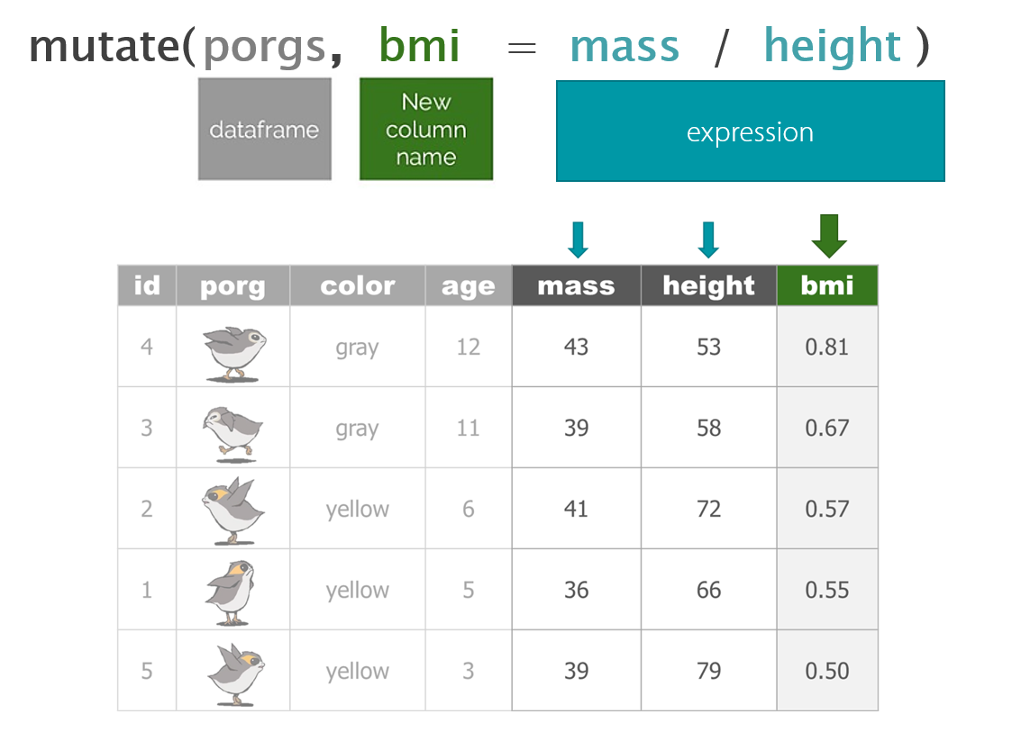
7 `mutate()`

mutate() can edit existing columns in a data frame or add new values that are calculated from existing columns.

Add a column

First, let’s add a column with our names. That way Rey can thank us personally when her ship is finally up and running.

# Add your name as a column
scrap <- mutate(scrap, scrap_finder = "BB8")

Add several columns

Let’s also add a new column to document the data measurement method.

#  Add your name as a column and
#  some information about the method
scrap <- mutate(scrap, 
                scrap_finder    = "BB8",
                measure_method  = "REM-24")

## REM = Republic Equivalent Method

Change a column

Remember how the units of Tons was written two ways: “TONS” and “Tons”? We can use mutate() together with tolower() to make sure all of the scrap units are written in lower case. This will help prevent them from getting grouped separately in our plots and summaries.

# Set units to all lower-case
scrap <- mutate(scrap, units = tolower(units))

# toupper() changes all of the letters to upper-case.

Add calculated columns

In our work we often use mutate to convert units for measurements. In this case, let’s estimate the total pounds for the scrap items that are reported in tons.

Tons `to` Pounds conversion

We can use mutate() to convert the amount column to pounds. Multiply the amount column by 2000 to get new values for a column named amount_lbs.

scrap_pounds <- mutate(scrap, amount_lbs = amount * 2000)

Final stretch!

We now have all the tools we need.

To get Rey’s ship working we need to track down more of the scrap item: Ion engine.

Step 1:

filter the data to only Ion engine

Show code

# Grab only the items named "Ion engine"
scrap_pounds <- filter(scrap_pounds, item == "Ion engine")

Next arrange the data in descending order of pounds so Rey knows where the highest amount of Ion engine scrap comes from.

Step 2:

arrange in descending order by amount_lbs

Show code

# Arrange data
scrap_pounds <- arrange(scrap_pounds, desc(amount_lbs))

# Return the origin of the highest amount_lbs of scrap
head(scrap_pounds, 1)

# Plot the total amount_lbs by origin
ggplot(scrap_pounds, aes(x = origin, y = amount_lbs)) + 
  geom_col()

Complete the mission!

For the item Ion engine, which origin has the most amount_lbs?

Tuanul
Cratertown
Outskirts
Reestki

Show solution

Cratertown

Yes!! You receive the ship parts to repair Rey’s Millennium Falcon. Onward!

First mission complete!

Nice work! Rey got a great deal on her engines and even traded in some scrap for spending cash. You’ve got the music in you, oh, oh, oh… Sorry.

Time to get off this dusty planet, we’re flying to Endor!

8 Save our data

You can’t break your original dataset if you name your edited data something new. Let’s use the readr package to save our new CSV with the tons converted to pounds.

# Save data as a CSV file 
write_csv(scrap_pounds, "scrap_in_pounds.csv")

Where did R save the file?

Hint: You can look in the lower right [Files] tab.

Let’s create a new results/ folder to keep our processed data separate from any raw data we receive. Now we can add results/ to our file path when we save the file.

# Save data as a CSV file to results folder
write_csv(scrap_pounds, "results/scrap_in_pounds.csv")

9 Plots with ggplot2

Plot the data, Plot the data, Plot the data

The `ggplot()` sandwich

A `ggplot` has 3 ingredients.

1. The base plot

library(ggplot2)

ggplot(scrap)

we load version 2 of the package library(ggplot2), but the function to make the plot is only ggplot(). No 2. Sorry.

2. The the X, Y aesthetics

The aesthetics assign the columns from the data that you want to use in the chart. This is where you set the X-Y variables that determine the dimensions of the plot.

ggplot(scrap, aes(x = origin, y = amount))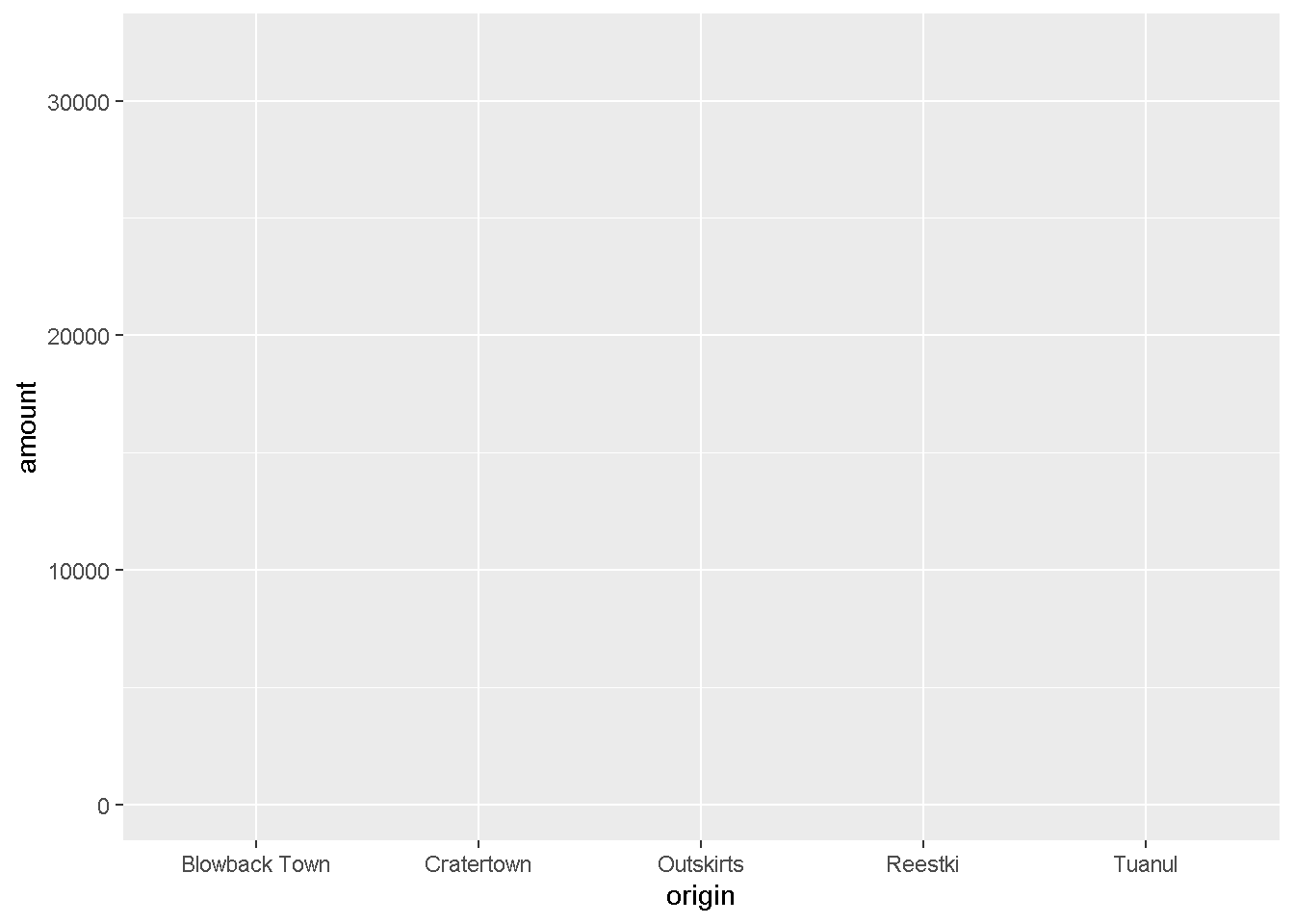

3. The layers or geometries

ggplot(scrap, aes(x = origin, y = amount)) + geom_col()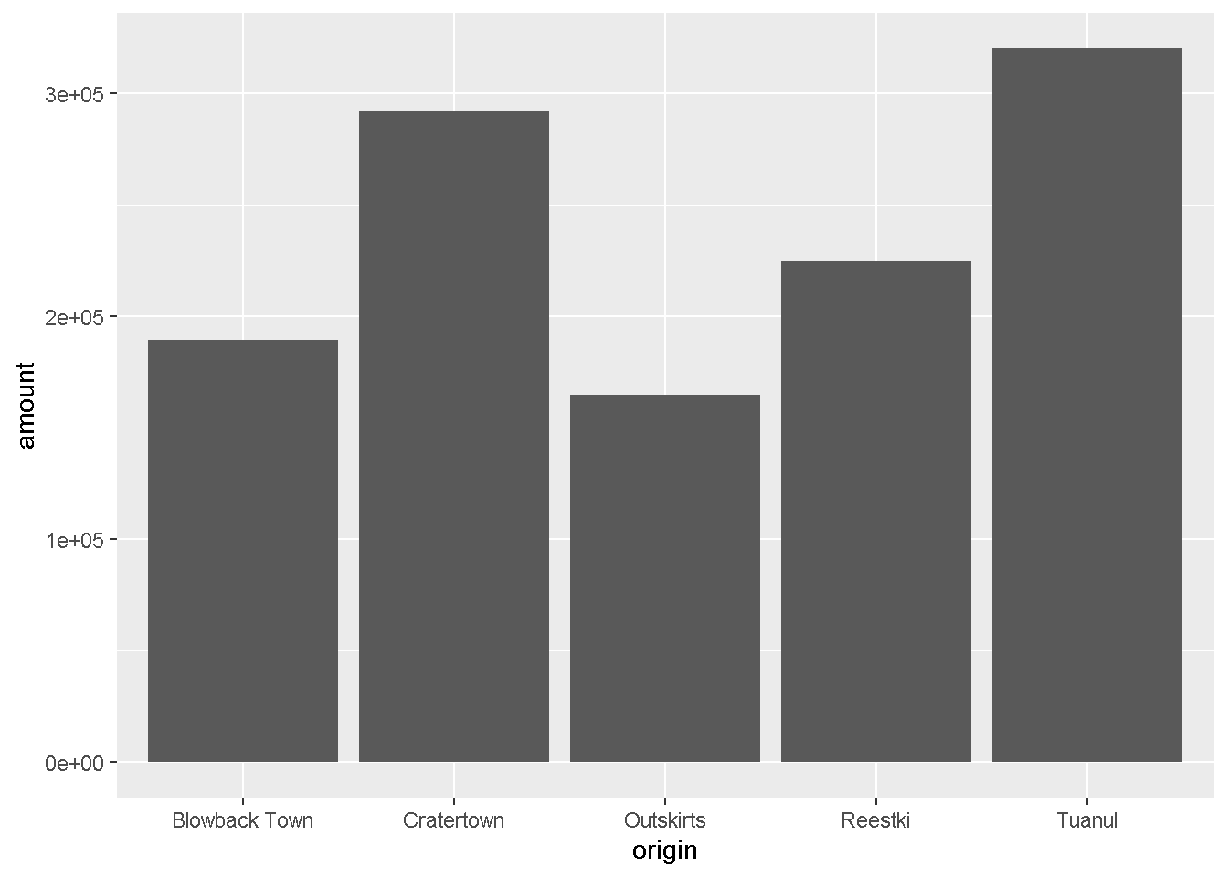

Colors

Now let’s change the fill color to match the origin.

ggplot(scrap, aes(x = origin, y = amount, fill = origin)) +
  geom_col()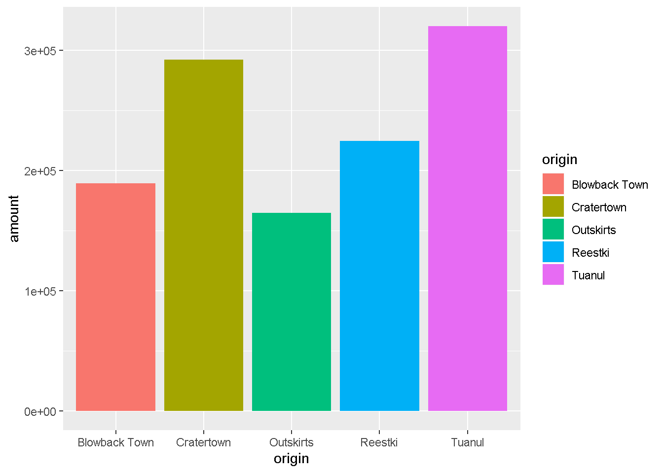

Explore!

Try making a column plot showing the total amount of scrap for each destination or for each item.

ggplot(scrap, aes(x = destination, y = amount )) + geom_col()

10 Shutdown complete

When you close R for the first time you’ll see some options about saving your workspace, history, and other files. In general, we advise against saving these files. This will help RStudio open a fresh and clean environment every time you start it. And it’s easy enough to re-run your script next time you open your project.

Follow these steps to set these options permanently, and not have to see the pop-up windows when you close R.

Turn off Save Workspace

Go to Tools > Global Options.... on the top RStudio navigation bar
On the first screen:
- [ ] Uncheck Restore .Rdata into workspace at startup
- Set Save workspace to .RData on exit to [“Never?].
- [ ] Uncheck Always save history

REVIEW: Functions & arguments

Functions perform steps based on inputs called arguments and usually return an output object. There are functions in R that are really complex but most boil down to the same general setup:

new_output <- function(argument_input1, argument_input2)

You can make your own functions in R and name them almost anything you like, even my_amazing_starwars_function().

You can think of a function like a plan for making Clone Troopers.

create_clones(host       = "Jango Fett", 
              n_troopers = 2000)

The function above creates Clone Troopers based on two arguments: the host and n_troopers. When we have more than one argument, we use a comma to separate them. With some luck, the function will successfully return a new object - a group of 2,000 Clone Troopers.

The sum() function

We can use the sum() function to find the sum age of our Star Wars characters.

starwars_ages  <- c(19,19,25)

# Call the sum function with starwars_ages as input
ages_sum <- sum(starwars_ages) # Assigns the output to starwars_ages_sum

# Print the starwars_ages_sum value to the console
ages_sum

## [1] 63

The sum() function takes the starwars_ages vector as input, performs a calculation, and returns a number. Note that we assigned the output to the name ages_sum.

If we don’t assign the output it will be printed to the console and not saved.

# Alternative without assigning output
sum(starwars_ages)

## [1] 63

Note

The original starwars_ages vector has not changed. Each function has its own “environment” and its calculations happen inside a bubble. In general, what happens inside a function won’t change your objects outside of the function.

starwars_ages

## [1] 19 19 25

New data -> New project!

It’s time for some Earth data. Use your new R skills to explore some data from closer to home.

Set up your project

Open a new project
Open a new R script
Create a data folder in your project directory
Copy your data to that folder

Begin your analysis

1. Read data into R

library(readr)
library(janitor)

# Read a CSV file
air_data <- read_csv("data/My-data.csv")


# Have an EXCEL file?
## You can use read_excel() from the readxl package
install.packages(readxl)

library(readxl)

# Read an EXCEL file
air_data <- read_excel("data/My-data.xlsx")

2. Clean the column names

air_data <- clean_names(air_data)

3. Get to know your data

Hint: summary(), glimpse(), nrow(), names()

4. Plot the data

library(ggplot2)

# Remember the ggplot sandwich!
ggplot(air_data, aes(x = TEMP_F, y = OZONE)) +
    geom_point(aes(color = site_name))

Keep exploring…

Data exploration

1 dplyr

Get to know your data frame

Data frame info

2 glimpse() & summary()

Let’s read the data into R and give these a whirl.

Explore!

Your analysis toolbox

3 Porg tables

4 select()

Drop columns with a minus sign: -col_name

Drop multiple columns

Keep only 3 columns

everything() else the same

5 Sort with arrange()

Big things first: desc()

Explore!

Spock-tip!

R BINGO!

6 filter()

Spock-tip!

Comparing values

Menu of comparisons

Explore!

6.1 Dropping rows

Multiple filters

7 mutate()

Add a column

Add several columns

Change a column

Add calculated columns

Tons to Pounds conversion

Final stretch!

Complete the mission!

First mission complete!

8 Save our data

9 Plots with ggplot2

Plot the data, Plot the data, Plot the data

The ggplot() sandwich

A ggplot has 3 ingredients.

1. The base plot

2. The the X, Y aesthetics

3. The layers or geometries

Colors

Explore!

10 Shutdown complete

Note

New data -> New project!

Set up your project

Begin your analysis

1. Read data into R

2. Clean the column names

3. Get to know your data

4. Plot the data

Return to Homebase

2 `glimpse()` & `summary()`

4 `select()`

Drop columns with a minus sign: `-col_name`

`everything()` else the same

5 Sort with `arrange()`

Big things first: `desc()`

6 `filter()`

7 `mutate()`

Tons `to` Pounds conversion

The `ggplot()` sandwich

A `ggplot` has 3 ingredients.