Good morning, Jedis!

Schedule
- Review of Day 1
- Dates continued...
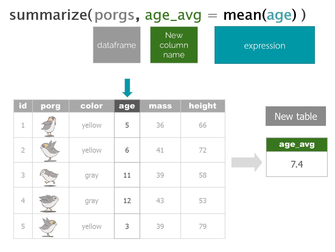
- Summarize your data
- Pipe together functions
- Join two tables by a shared column
- Calculate new columns
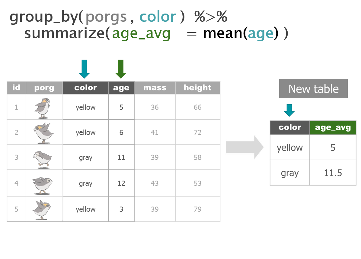
- Summarize for each group
- Save dataPorg review
The poggle of porgs has returned to help review the dplyr functions. Follow along by downloading the porg data from the URL below.
library(readr)
porgs <- read_csv("https://itep-r.netlify.com/data/porg_data.csv")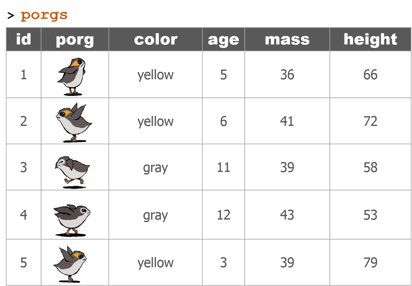


1 New mission!
The Wookies want our help. BB8 just received new data from the wookies suggesting there was a large magnetic storm just before Site 1 burned down on Endor. Sounds like we’re going to be STORM CHASERS! Mission accepted.
Get the dataset
While we’re relaxing and flying to Endor let’s get set up with the new data.
Endor setup
- Download the data.
- DOWNLOAD - Get the Endor monitoring data
- Create a new folder called
datain your project folder. - Move the downloaded Endor file to there.
- Create a new R script called
endor.R
Now we can read in the data from the data folder with our favorite read_csv function.
library(readr)
library(dplyr)
library(janitor)

air_endor <- read_csv("data/air_endor.csv")

names(air_endor)

# Clean the column names
air_endor <- clean_names(air_endor)

names(air_endor)
## [1] "analyte" "lab_code" "units" "start_run_date"
## [5] "site_name" "long_site_name" "planet" "result"Note
When your project is open, RStudio sets the working directory to your project folder. When reading files from a folder outside of your project, you’ll need to use the full file path location.
For example, for a file on the X-drive: X://Programs/Air_Quality/Ozone_data.csv
Welcome to Endor!

Let’s get to know the Endor data.
Remember the ways?
Hint: summary(), glimpse(), nrow(), distinct()
glimpse(air_endor)## Observations: 1,190
## Variables: 8
## $ analyte <chr> "1-Methylnaphthalene", "1-Methylnaphthalene", "...
## $ lab_code <chr> "HV-403", "HV-408", "HV-411", "HV-415", "HV-418...
## $ units <chr> "ng/m3", "ng/m3", "ng/m3", "ng/m3", "ng/m3", "n...
## $ start_run_date <chr> "7/11/2016", "7/23/2016", "8/5/2016", "8/16/201...
## $ site_name <chr> "battlesite1", "battlesite1", "battlesite1", "b...
## $ long_site_name <chr> "Endor_Tana_forestmoon_battlesite1", "Endor_Tan...
## $ planet <chr> "Endor", "Endor", "Endor", "Endor", "Endor", "E...
## $ result <dbl> 0.00291, 0.00000, 0.00000, 0.00608, 0.00000, 0....distinct(air_endor, analyte)## # A tibble: 27 x 1
## analyte
## <chr>
## 1 1-Methylnaphthalene
## 2 2-Methylnaphthalene
## 3 5-Methylchrysene
## 4 Acenaphthene
## 5 Anthanthrene
## 6 Benz[a]anthracene
## 7 Benzo[a]pyrene
## 8 Benzo[c]fluorene
## 9 Benzo[e]pyrene
## 10 Benzo[g,h,i]perylene
## # ... with 17 more rowsWoah! That’s definitely more analytes than we need.
We only want to know about magnetic_field data. Let’s filter down to that analyte.
mag_endor <- filter(air_endor, analyte == "magnetic_field")Boom! How many rows are left now?
Ok. According to the request we received, the Resistance is only interested in observations from year
2017. So let’s filter the data down to only dates for that year.How do we filter on the date column?
With time series data it’s helpful for R to know which columns are dates. Dates come in many formats and the standard format in R is 2019-01-15, also referred to as Year-Month-Day format. We use the lubridate package to help format our dates.
2 Dates
Enter the lubridate package.

It’s about time! Lubridate makes working with dates much easier.
We can find how much time has elapsed, add or subtract days, and find seasonal and day of the week averages.
Convert text to a DATE
| Function | Order of date elements |
|---|---|
mdy() |
Month-Day-Year :: 05-18-2019 or 05/18/2019 |
dmy() |
Day-Month-Year (Euro dates) :: 18-05-2019 or 18/05/2019 |
ymd() |
Year-Month-Day (science dates) :: 2019-05-18 or 2019/05/18 |
ymd_hm() |
Year-Month-Day Hour:Minutes :: 2019-05-18 8:35 AM |
ymd_hms() |
Year-Month-Day Hour:Minutes:Seconds :: 2019-05-18 8:35:22 AM |
Get date parts
| Function | Date element |
|---|---|
year() |
Year |
month() |
Month as 1,2,3; For Jan, Feb, Mar use label=TRUE |
week() |
Week of the year |
day() |
Day of the month |
wday() |
Day of the week as 1,2,3; For Sun, Mon, Tue use label=TRUE |
| - Time - | |
hour() |
Hour of the day (24hr) |
minute() |
Minutes |
second() |
Seconds |
tz() |
Time zone |
Install lubridate
Run: install.packages("lubridate")
Clean the dates
Real world examples
Does your date column look like one of these? Here’s the lubridate function to tell R that the column is a date.
| Format | Function to use |
|---|---|
| “05/18/2019” | mdy(date_column) |
| “May 18, 2019” | mdy(date_column) |
| “05/18/2019 8:00 CDT” | mdy_hm(date_column, tz = "US/Central") |
| “05/18/2019 11:05:32 PDT” | mdy_hms(date_column, tz = "US/Pacific") |
European dates
| Format | Function to use |
|---|---|
| “30.05.2019” | dmy(date_column) |
| “30-05-2019” | dmy(date_column) |
| “30/05/2019” | dmy(date_column) |
AQS formatted dates
| Format | Function to use |
|---|---|
| “20190518” | ymd(sample_date) |
Small problem

Oh no! BB8 got locked out of the system! You need the passcode before you can unlock the data.
There’s a cryptic note on the pad next to you… “Marty’s birthday”. Could that be the hint to the passcode???
We need to determine when Marty’s birthday is…time to get out our detective hats.
You ask the lead engineer:
So when is Marty’s birthday?
“I think it’s on a Tuesday this year”
Any more helpful clues? Anything?
“Hmmm… Let’s see, I think it was around the 22nd week of the year. Yep. That’s it.”
Explore!
After some more interviews you now have a list of dates that could be Marty’s birthday. Find the date that occurred on the Tuesday of the 22nd week of the year.
library(lubridate)

date1 <- "7/2/2019"

date2 <- "28/05/2019"

date3 <- "June 4th, 2019"
Step 1: Use mdy(date) or dmy(date) to convert the dates to the universal date format.
Are you sure you want to click this button? There’s no going back.
Show code
# Use mdy() or dmy() to format dates

#1
date1 <- mdy("7/2/2019")

#2
date2 <- dmy("28/05/2019")

#3
date3 <- mdy("June 4th, 2019")
Step 2: Find the day of the week using wday(date), and week of the year using week(date).
Show code
# Use wday() and week() to get date info

#1
date1 <- mdy("7/2/2019")
wday(date1, label = TRUE, abbr = FALSE)
week(date1)

#2
date2 <- dmy("28/05/2019")
wday(date2, label = TRUE, abbr = FALSE)
week(date2)

#3
date3 <- mdy("June 4th, 2019")
wday(date3, label = TRUE, abbr = FALSE)
week(date3)
Show answer
"28/05/2019" or May 28th, 2019
Congrats! BB8 successfully accessed the backup system. The data is back online!
Back on Endor!
Let’s use the mdy() function to turn the start_run_date column into a nicely formatted date.
library(lubridate)

mag_endor <- mutate(mag_endor, date = mdy(start_run_date),
                               year = year(date))
Ok, back to work.
Let’s filter to only the rows where the
yearequals2017.
mag_endor <- filter(mag_endor, year == 2017)Time series
library(ggplot2)

ggplot(mag_endor, aes(x = date, y = result)) +
  geom_line(size = 2, color = "tomato") +
  geom_point(size = 5, alpha = 0.5)  # alpha changes transparency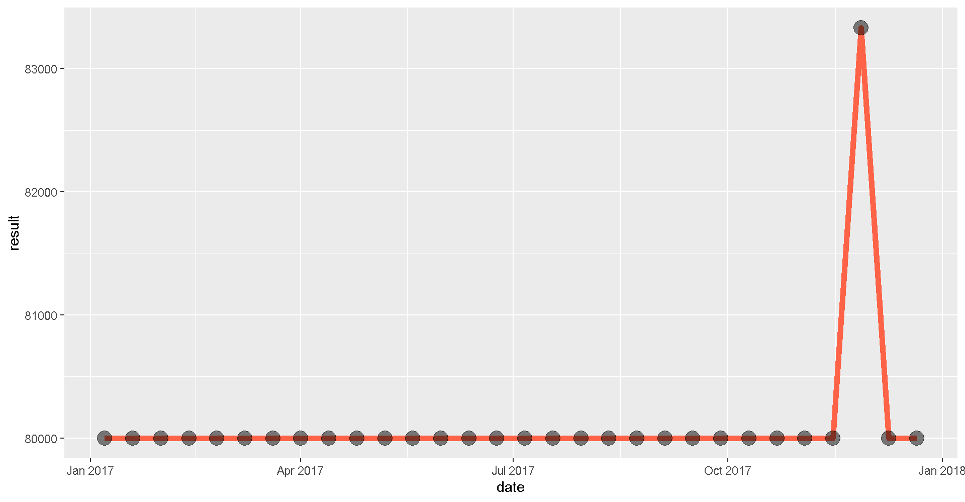
Looks like the measurements definitely picked up a signal towards the end of the year.
Mystery solved!
Aha! There really was a spike in the magnetic field in November. Hopefully, the Resistance will reward us handsomely for this information.
3 Calendar plots

Calendar plots are good for zooming in to see specific days when elevated observations may have occurred. Maybe we can pinpoint what day that magnetic storm may have occurred.
openair package
There is a calendar plot function in the package openair. Let’s install openair, load it, and use calendarplot() to make a calendar of the observations.
install.packages("openair")library(openair)calendarPlot(mag_endor,
pollutant = "result",
statistic = "mean",
year = 2017,
annotate = "date",
digits = 0,
key.footer = "nT",
par.settings = list(fontsize = list(text = 14),
layout.heights = list(top.padding = 1)),
main = "Magnetic Field Strength at Endor Battle Site 1")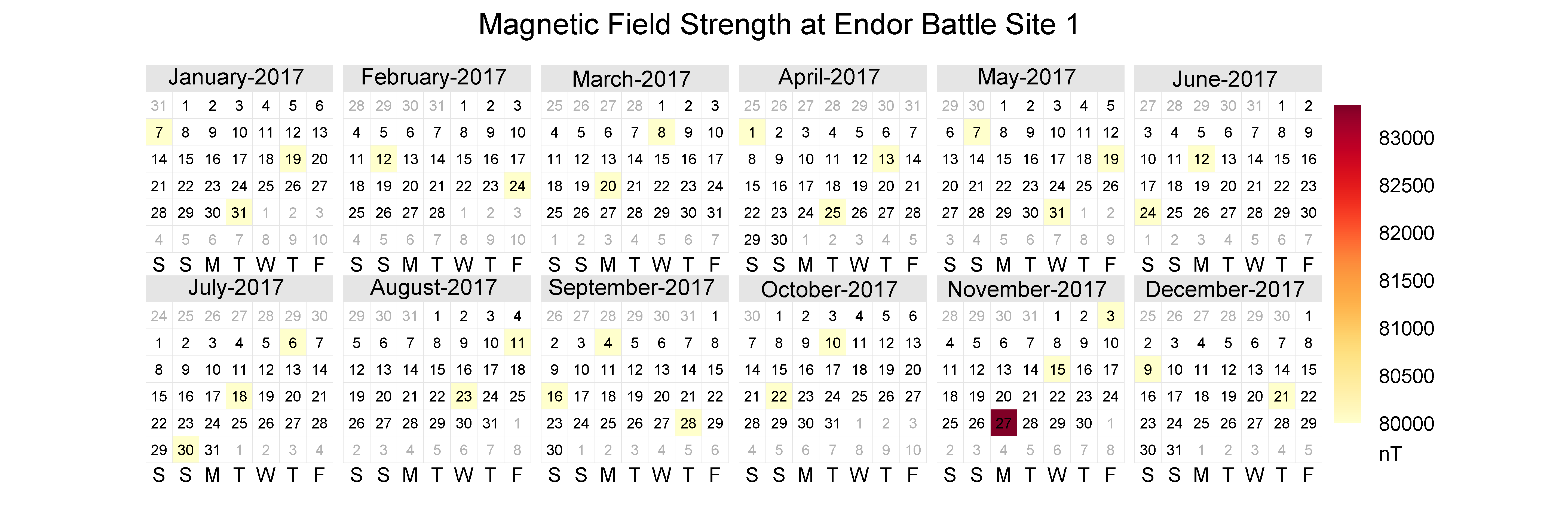
Let’s zoom in and filter the calendar to only 3 months: October, November, December.
mag_endor <- mutate(mag_endor, month = month(date))
mag_endor <- filter(mag_endor, month %in% c(10,11,12))
calendarPlot(mag_endor,
             pollutant    = "result",
             statistic    = "mean",
             year         = 2017,
             annotate     = "date",
             digits       = 0,
             key.footer   = "nT",
             par.settings = list(fontsize       = list(text = 14),
                                 layout.heights = list(top.padding = 1)),
             main = "Magnetic Field Strength at Endor Battle Site 1")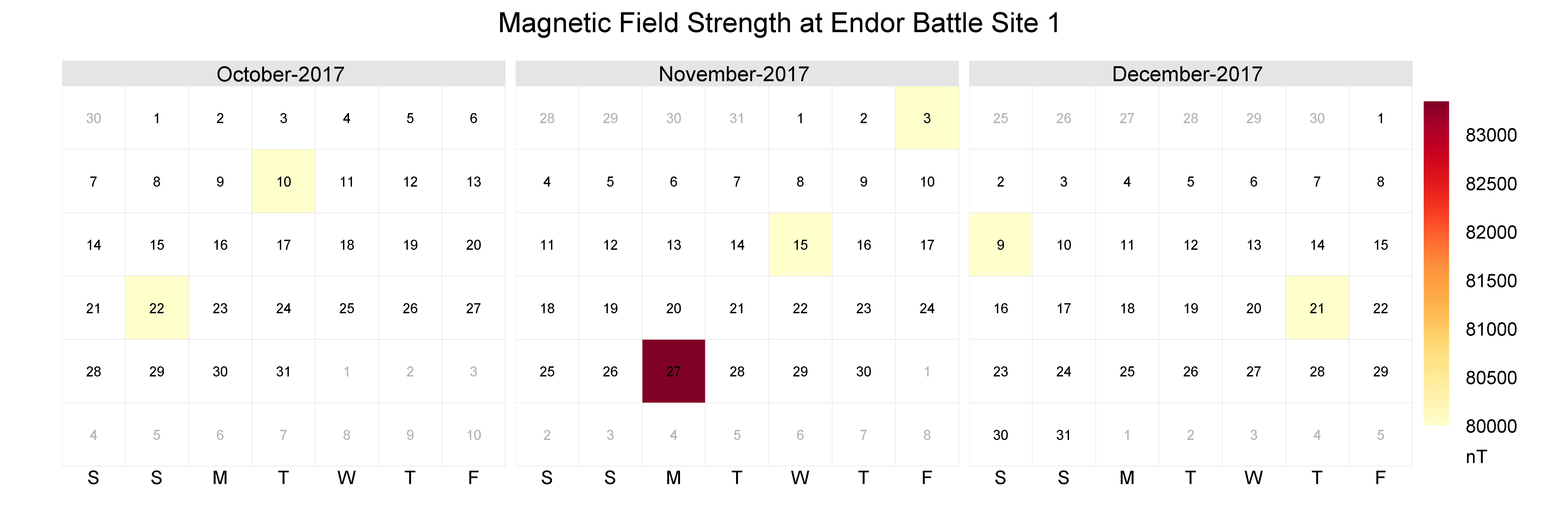
4 Pipe it together: A %>% B
Let the %>% guide you.
I wish I could type the name of the data less often.

You can with the pipe!
Use the %>% to chain functions together and make our scripts more streamlined.
Here are 2 ways the %>% is helpful:
#1: It eliminates the need for nested parentheses.
Say you wanted to take the sum of 3 numbers and then take the log and then round the final result.
round(log(sum(c(10, 20, 30, 50))))The code doesn’t look much like the words we used to describe it. Let’s pipe it so we can read the code from left to right.
c(10, 20, 30, 50) %>% sum() %>% log() %>% round()#2: We can combine many processing steps into one cohesive chunk.
Here are some of the functions we’ve applied to the scrap data so far:
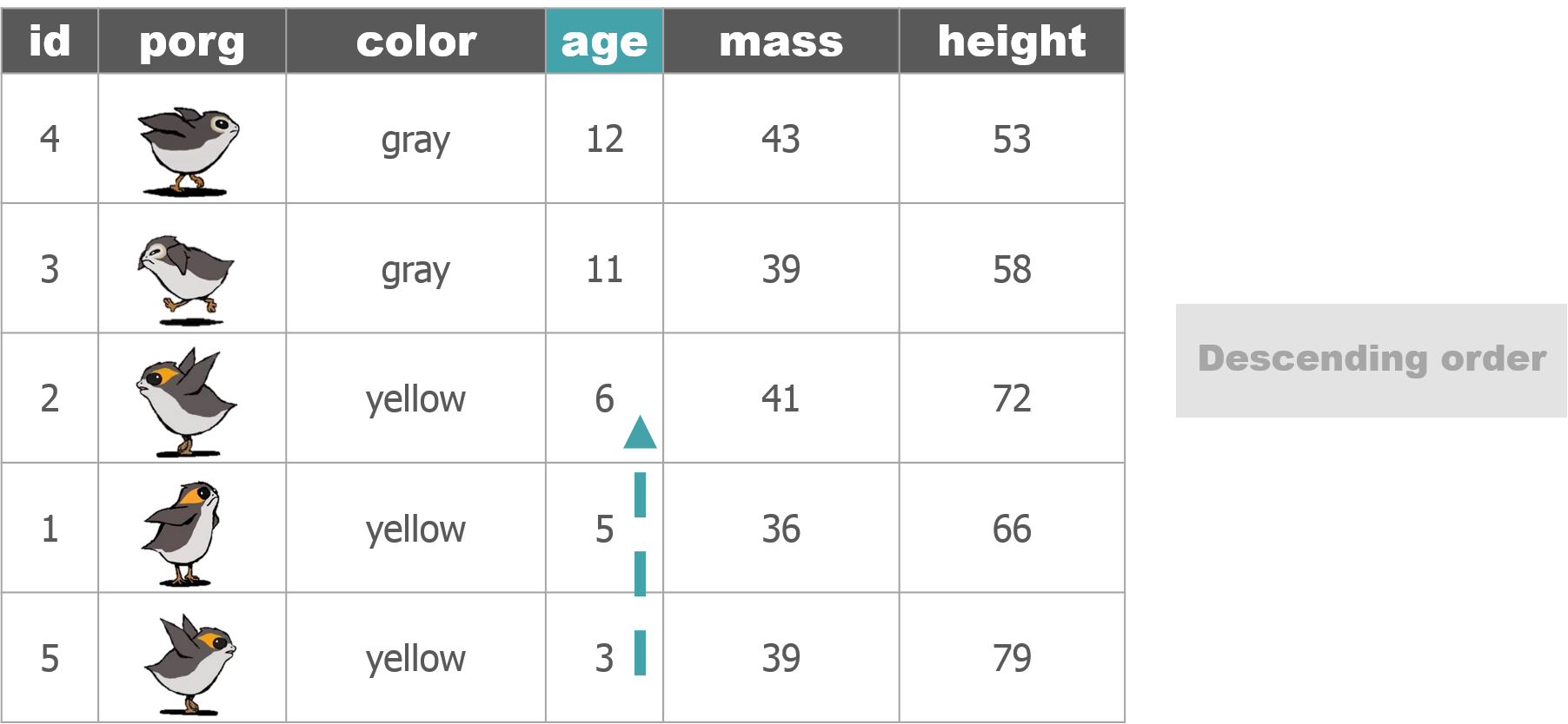
scrap <- arrange(scrap, desc(price_per_pound))

scrap <- filter(scrap, origin != "All")

scrap <- mutate(scrap,
                scrap_finder    = "BB8",
                measure_method  = "REM-24")
We can use the %>% operator to pipe or chain them together.
scrap <- scrap %>%
           arrange(desc(price_per_pound)) %>%
           filter(origin != "All") %>%
           mutate(scrap_finder    = "BB8",
                  measure_method  = "REM-24")
Explore!
Similar to above, use the %>% to combine the two Endor lines below.
# Filter to only magnetic_field measurements
mag_endor <- filter(air_endor, analyte == "magnetic_field")

# Add a date column to the filtered data
mag_endor <- mutate(mag_endor, date = mdy(start_run_date))
So where were we?
Right! We we’re enjoying our time on beautiful lush Endor. But aren’t we missing somebody…?
Finn needs us!
That’s enough scuttlebutting on Endor, Finn needs us back on Jakku. It turns out we forgot to pick-up Finn when we left. Now he’s being held ransom by Junk Boss Plutt. We’ll need to act fast to get to him before the Empire does. Blast off!

Update from BB8!
BB8 was busy on our flight back to Jakku, and recovered a full set of scrap records from the notorious Unkar Plutt. Let’s take a look.
library(readr)
library(dplyr)

# Read in the full scrap database
scrap <- read_csv("https://itep-r.netlify.com/data/starwars_scrap_jakku_full.csv")
5 Jakku re-visited
Okay, so we’re back on this ol’ dust bucket. Let’s try not to forget anyone this time. We’re quickly running out of friends on this planet.
A scrappy ransom
Mr. Baddy Plutt is demanding 10,000 items of scrap for Finn. Sounds expensive, but lucky for us he didn’t clarify the exact items. Let’s find the scrap that weighs the least per shipment and try to make this transaction as light as possible.
Take a look at our NEW scrap data and see if we have the weight of all the items.
# What unit types are in the data?
unique(scrap$units)
## [1] "Cubic Yards" "Items" "Tons"Or return results as a data frame
distinct(scrap, units)## # A tibble: 3 x 1
## units
## <chr>
## 1 Cubic Yards
## 2 Items
## 3 TonsHmmm…. So how much does a cubic yard of Hull Panel weigh?
A lot? 32? Maybe…
I think we’re going to need some more data.
“Hey BB8!”
“Do your magic data finding thing.”
Weight conversion

It took a while, but with a few droid bribes BB8 was able to track down a Weight conversion table from his droid buddies. Our current data shows the total cubic yards for some scrap shipments, but not how much the shipment weighs.
Read the weight conversion table
# The data's URL
convert_url <- "https://rtrain.netlify.com/data/conversion_table.csv"

# Read the conversion data
convert <- read_csv(convert_url)

head(convert, 3)
## # A tibble: 3 x 3
## item units pounds_per_unit
## <chr> <chr> <dbl>
## 1 Bulkhead Cubic Yards 321
## 2 Hull Panel Cubic Yards 641
## 3 Repulsorlift array Cubic Yards 467Stars! A cubic yard of Hull Panel weighs 641 lbs. That’s what I thought!
Let’s join this new conversion table to the scrap data to make our calculations easier. To do that we need to make a new friend.
Say Hello to left_join()!
6 Join tables with left_join()
Join 2 tables
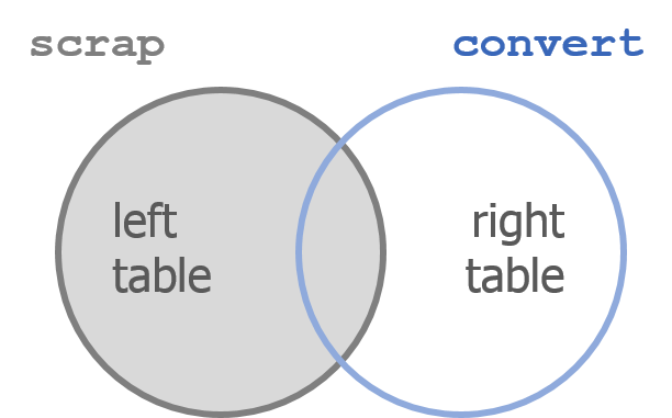
left_join(scrap, convert, by = c("columns to join by"))
left_join() works like a zipper to combine 2 tables based on one or more variables. It’s called “left”-join because the entire table on the left side is retained.
Anything that matches from the right table gets to join the party, but any rows that don’t have a matching ID will be ignored.
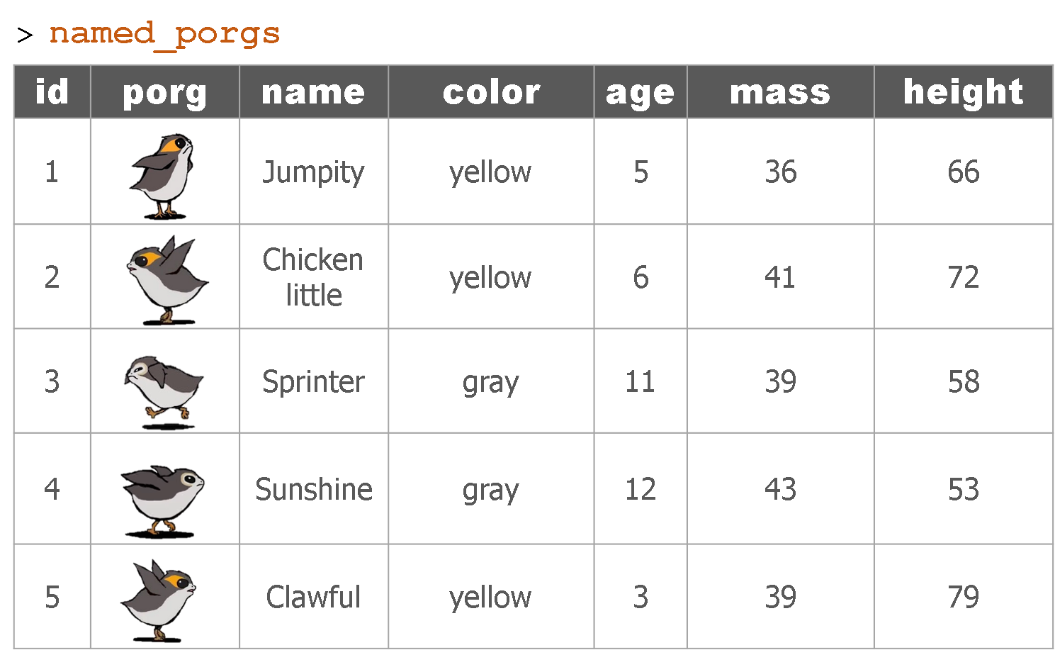
Adding porg names
Remember our porg friends? How rude of us not to share their names. Wups!
Here’s a table of their names.
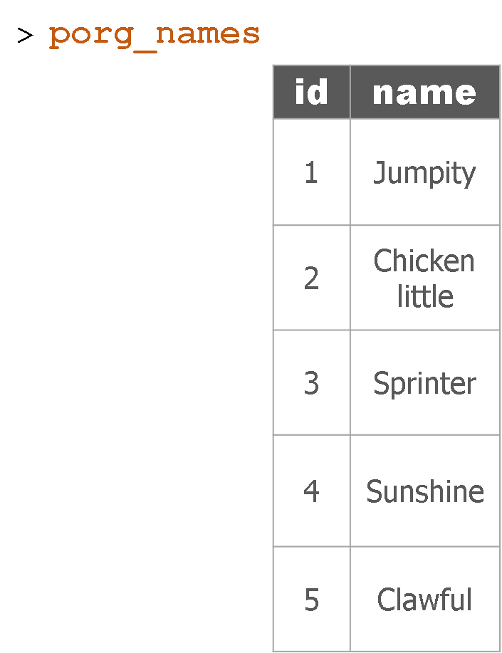
Hey now! Who’s who? Let’s join their names to the rest of the data.
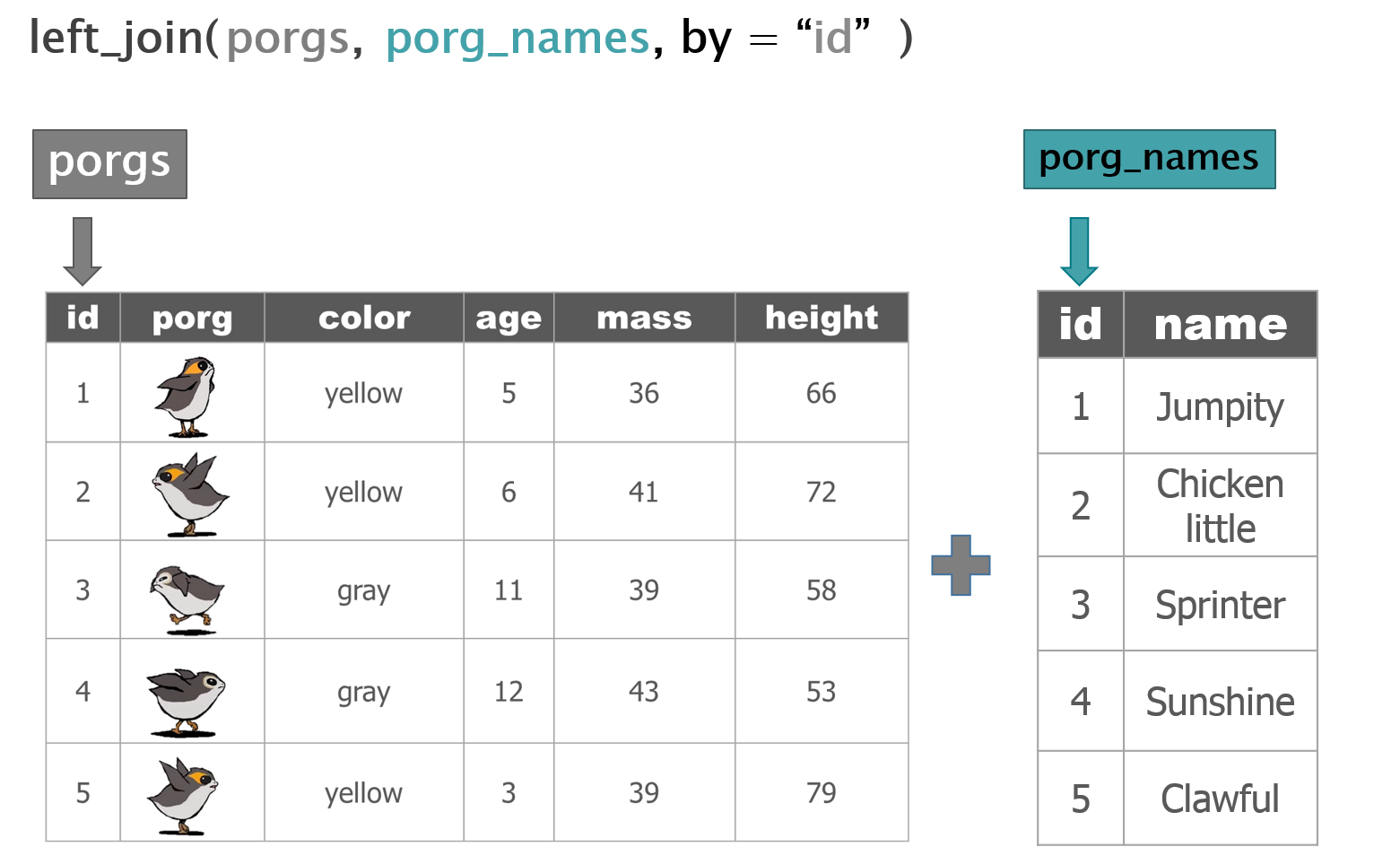
The joined result:
BONUS More joining
Star Wars characters
left_join() is used to add columns to your table by pulling them from another table. Imagine you have the 2 Star Wars tables below. One table includes character names and heights; the second has names and homeworlds. Since both tables share a common name column, we can join the tables together using the name columns as the joining key.
starwars_heights
| starwars_name | height |
|---|---|
| Luke Skywalker | 172 |
| C-3PO | 167 |
| Darth Vader | 202 |
| Leia Organa | 150 |
| Greedo | 246 |
starwars_homeworlds
| starwars_name | homeworld |
|---|---|
| Luke Skywalker | Tatooine |
| C-3PO | Tatooine |
| Darth Vader | Tatooine |
| Leia Organa | Alderaan |
| Ayla Secura | Ryloth |
Uh oh! There’s no “Ayla Secura” in the height table and there’s no “Greedo” in the homeworld table. Can we still join the tables? Run the code below to see what happens.
library(dplyr)

# Create new tables
starwars_heights <- data_frame(starwars_name = c("Luke Skywalker", "C-3PO", "Darth Vader", "Leia Organa", "Greedo"),
                               height = c(172, 167, 202, 150, 246))

starwars_homeworlds <- data_frame(starwars_name = c("Luke Skywalker", "C-3PO", "Darth Vader", "Leia Organa", "Ayla Secura"),
                                  homeworld = c("Tatooine", "Tatooine", "Tatooine", "Alderaan", "Ryloth"))

# Join the tables together by starwars_name
## Tell left_join which columns to use as the key with:
##     by = c("key_left" = "key_right")
height_and_homeworld <- left_join(starwars_heights, starwars_homeworlds,
                                  by = c("starwars_name" = "starwars_name"))

height_and_homeworld| starwars_name | height | homeworld |
|---|---|---|
| Luke Skywalker | 172 | Tatooine |
| C-3PO | 167 | Tatooine |
| Darth Vader | 202 | Tatooine |
| Leia Organa | 150 | Alderaan |
| Greedo | 246 | NA |
Did it work?
When left_join adds the homeworlds column to the starwars_heights table it only adds a value for the characters when the tables have a matching character name. When R couldn’t find “Greedo” in the homeworld table, the Star Wars character’s homeworld was recorded as missing or NA.
Multiple records

Now imagine the table starwars_homeworld has two records for C-3PO, each with a different homeworld listed.
What will happen when you join the two tables?
starwars_heights
| starwars_name | height |
|---|---|
| Luke Skywalker | 172 |
| C-3PO | 167 |
| Darth Vader | 202 |
| Leia Organa | 150 |
| Greedo | 246 |
starwars_homeworlds
| starwars_name | homeworld |
|---|---|
| Luke Skywalker | Tatooine |
| C-3PO | Tatooine |
| C-3PO | Tantive IV |
| Darth Vader | Tatooine |
| Leia Organa | Alderaan |
| Ayla Secura | Ryloth |
When you run the code below you’ll see that left_join is very thorough and adds each additional homeworld it finds for C-3PO as a new row in the joined table.
# Create new tables
starwars_heights <- data_frame(starwars_name = c("Luke Skywalker", "C-3PO", "Darth Vader", "Leia Organa", "Greedo"),
                               height  = c(172, 167, 202, 150, 173))


starwars_homeworlds <- data_frame(starwars_name = c("Luke Skywalker", "C-3PO", "C-3PO", "Darth Vader", "Leia Organa", "Ayla Secura"),
                                  homeworld = c("Tatooine", "Tatooine", "Tantive IV", "Tatooine", "Alderaan", "Ryloth"))

# Join the tables together by Star Wars character name
height_and_homeworld <- left_join(starwars_heights, starwars_homeworlds)

# Check number of rows
nrow(height_and_homeworld)

height_and_homeworld| starwars_name | height | homeworld |
|---|---|---|
| Luke Skywalker | 172 | Tatooine |
| C-3PO | 167 | Tatooine |
| C-3PO | 167 | Tantive IV |
| Darth Vader | 202 | Tatooine |
| Leia Organa | 150 | Alderaan |
| Greedo | 173 | NA |
This results in a table with one extra row than we started with in our heights table. So growing table sizes are a sign of duplicate records when using left_join().
In practice, when you see this you’ll want to investigate why one of your tables has duplicate entries, especially if the observation for the two rows is different, as it was for C-3PO’s homeword.
Are there really two different Star Wars characters named C-3PO, or maybe someone made two different guesses about the droid’s homeworld, or maybe the data simply has a mistake.
Back to the scrap yard
Let’s apply our new left_join() skills to the scrap data.
First, let’s re-read the full scrap data.
library(readr)
library(dplyr)

# Read in the larger scrap database
scrap <- read_csv("https://itep-r.netlify.com/data/starwars_scrap_jakku_full.csv")

# what units types are in the data?
distinct(scrap, units)
## # A tibble: 3 x 1
## units
## <chr>
## 1 Cubic Yards
## 2 Items
## 3 TonsJoin the conversion table to scrap
Look at the tables. What columns in both tables do we want to join by?
names(scrap)Let’s join by item and units.
# Join the scrap to the conversion table
scrap <- left_join(scrap, convert,
                   by = c("item"  = "item",
                          "units" = "units"))
Want to save on typing?
left_join() will automatically search for matching columns if you don’t use the by= argument. So if you know 2 tables share a column name you don’t have to specify how to join them. The code below does the same as above.
scrap <- left_join(scrap, convert)

head(scrap, 4)
## # A tibble: 4 x 8
## receipt_date item origin destination amount units price_per_pound
## <chr> <chr> <chr> <chr> <dbl> <chr> <dbl>
## 1 4/1/2013 Bulk~ Crate~ Raiders 4017 Cubi~ 1005.
## 2 4/2/2013 Star~ Outsk~ Trade cara~ 1249 Cubi~ 1129.
## 3 4/3/2013 Star~ Outsk~ Niima Outp~ 4434 Cubi~ 1129.
## 4 4/4/2013 Hull~ Crate~ Raiders 286 Cubi~ 843.
## # ... with 1 more variable: pounds_per_unit <dbl>Help!
For more details, you can type ?left_join to see all the arguments and options.
Total pounds per shipment
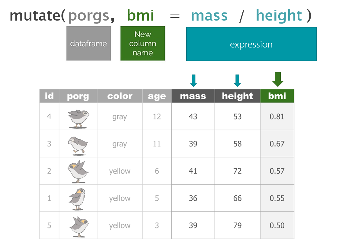
Let’s mutate()!
Now that we have pounds per unit we can use mutate to calculate the total pounds for each shipment.
Fill in the blank
scrap <- scrap %>%
         mutate(total_pounds = amount *  _____________ )
Show code
scrap <- scrap %>%
         mutate(total_pounds = amount * pounds_per_unit)
Total price per shipment
Explore!
Total price
We need to do some serious multiplication. We now have the total amount shipped in pounds, and the price per pound, but we want to know the total price for each transaction.
How do we calculate that?
# Calculate the total price for each shipment
scrap <- scrap %>%
         mutate(credits = ________ * ________ )
Total price
We need to do some serious multiplication. We now have the total amount shipped in pounds, and the price per pound, but we want to know the total price for each transaction.
How do we calculate that?
# Calculate the total price for each shipment
scrap <- scrap %>%
         mutate(credits = total_pounds  * ________ )
Total price
We need to do some serious multiplication. We now have the total amount shipped in pounds, and the price per pound, but we want to know the total price for each transaction.
How do we calculate that?
# Calculate the total price for each shipment
scrap <- scrap %>%
         mutate(credits = total_pounds * price_per_pound)
Price per item
Great! Let’s add one last column. We can divide the shipment’s credits by the amount of items to get the price_per_unit.
# Calculate the price per unit
scrap <- scrap %>%
         mutate(price_per_unit = credits / amount)
Note
Analysts often get asked questions:
- What’s the highest number?
- What’s the lowest number?
- What was the average tons of scrap from Cratertown last year?
- Which town’s scrap was worth the most credits?