
Remember what you should do first when you start your R session? First we load the packages we will need.
#Load packages

library(readr)
library(dplyr)
library(ggplot2)
Start by reading in the data. It is a clean version of the scrap data we’ve been using.
Notice that we are including comments in the R script so that your future self can follow along and see what you did.
Read in data
clean_scrap <- read_csv("https://itep-r.netlify.com/data/starwars_scrap_jakku_clean.csv")

head(clean_scrap)
## # A tibble: 6 x 6
## items origin destination price_per_ton amount_tons total_price
## <chr> <chr> <chr> <dbl> <dbl> <dbl>
## 1 electroteles~ outskirts trade cara~ 850. 868. 737981.
## 2 atmospheric ~ craterto~ niima outp~ 56.2 33978. 1909912.
## 3 bulkhead craterto~ raiders 1005. 645. 647843.
## 4 main drive blowback~ trade cara~ 598. 1961. 1172184.
## 5 flight recor~ outskirts niima outp~ 591. 887 524155.
## 6 proximity se~ outskirts raiders 1229. 7081 8702761.Did it load successfully? Look in your environment. You should see “clean_scrap”. There should be 6 variables and 573 rows.
Take a couple of minutes to get an overview of the data. Open and look at your data in at least two ways. Do you remember some of the functions to do that?
1. Click on the data name in the environment to open the window. 1. Use glimpse() to look at your data.
Show solution
#View the data
glimpse(clean_scrap)
## Observations: 573
## Variables: 6
## $ items <chr> "electrotelescope", "atmospheric thrusters", "bu...
## $ origin <chr> "outskirts", "cratertown", "cratertown", "blowba...
## $ destination <chr> "trade caravan", "niima outpost", "raiders", "tr...
## $ price_per_ton <dbl> 849.79, 56.21, 1004.83, 597.85, 590.93, 1229.03,...
## $ amount_tons <dbl> 868.4280, 33978.1545, 644.7285, 1960.6650, 887.0...
## $ total_price <dbl> 737981.43, 1909912.06, 647842.54, 1172183.57, 52...Look at a summary of your data using summary().
Show solution
#View a summary of the data
summary(clean_scrap)
## items origin destination
## Length:573 Length:573 Length:573
## Class :character Class :character Class :character
## Mode :character Mode :character Mode :character
##
##
##
## price_per_ton amount_tons total_price
## Min. : 29.15 Min. : 0.01 Min. : 5
## 1st Qu.: 314.23 1st Qu.: 238.99 1st Qu.: 128921
## Median : 629.28 Median : 1298.00 Median : 757656
## Mean :1010.85 Mean : 3724.23 Mean : 3483802
## 3rd Qu.:1329.05 3rd Qu.: 4678.44 3rd Qu.: 2631778
## Max. :7211.01 Max. :60116.67 Max. :83712615
What if you only want to keep the items and amount_tons fields? Use select() to create a new data frame keeping only those columns and save it as an object called
select_scrap.
Show solution
select_scrap <- select(clean_scrap, items, amount_tons)Order the data frame you just created by amount_tons from highest to lowest. Which item had the highest weight?
Show solution
select_scrap <- arrange(select_scrap, desc(items))Filter your select data set to all items with an amount higher than 1000. Call the dataset ‘filter_scrap’
Show solution
filter_scrap <- filter(select_scrap, amount_tons > 1000)Add a filter to to the amount_tons > 1000 dataset. Include only “proximity sensor” and “hyperdrive”
Show solution
You will need %in%, c() and filter.
Show solution
filter_scrap <- filter(select_scrap, amount_tons > 1000,
                       items %in% c("proximity sensor", "hyperdrive"))
Add a column with your favorite Star Wars character to your filtered data frame.
Show solution
filter_scrap <- mutate(filter_scrap, my_favorite_character = "Admiral Ackbar")We’ve got all the amount of items in tons in our data set, and we have our favorite StarWars character, but we want to include the amount of items in pounds. Use mutate() to calculate the number of pounds in your filtered dataset. Call that column ‘amount_pounds’.
Show solution
filter_scrap <- mutate(filter_scrap, amount_pounds = amount_tons * 2000)We want to make a table of recommendations to our Junk Boss Unkar Plutt. In our filtered dataset, we want to buy scrap if if it is a
Hyperdriveand ignore scrap if its aProximity sensor. Remember, we filtered our table to only those two types of scrap. Use mutate() to make a column that reports “buy” if the item is ahyperdriveand “ignore” if the item is aproximity sensor. Call this new columndo_this. You will need both ifelse() and mutate() for this task.
Show solution
filter_scrap <- mutate(filter_scrap, do_this = ifelse(items == "hyperdrive", "buy", "ignore"))
> Let’s take a closer look at our full dataset now (clean_scrap). We want to give the Junk Boss a summary of all of this data. He doesn’t have the patience to really look at a lot of data. He hates numbers! He likes money. He wants to know the following things:
- The sum of all the money potentially earned by item.
- The maximum money potentially earned by item.
- The number of reports of each item.
- The 35th percentile of the price by item.
[We don’t even know how he learned about “quantile”, we are pretty sure someone told him about this just to test our abilities. If we don’t provide this summarized dataset, Unkar Plutt is likely going to shoot us into space rendering us…dead. We don’t want that. Let’s make a summary table.]
Hint:
You will need the pipe %>%, group_by(), summarise(), sum(), max(), quantile(), and n().
Hint # 2!
summary_scrap <- clean_scrap %>%
                group_by() %>%
                summarise()
Show solution
summary_scrap <- clean_scrap %>%
  group_by(items) %>%
  summarise(sum_price = sum(total_price),
            max_price = max(total_price),
            count_price = n(),
            price_35th = quantile(total_price, 0.35))
Oh boy, old Unkar just learned about plots. What will he want next? He wants a plot of the maximum total prices by item. We must create this plot or perish. Try both geom_col() and geom_point(0) to see which make a more simple look at the price maxima.
Show solution
ggplot(data = summary_scrap, aes(items, max_price)) +
  geom_col()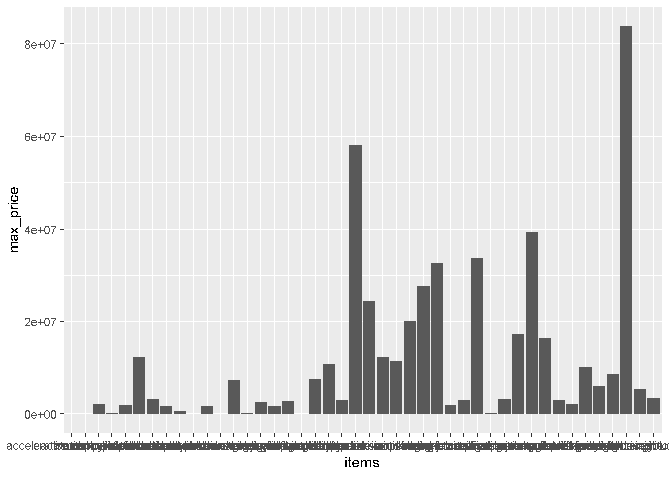
Show solution
ggplot(data = summary_scrap, aes(items, max_price)) +
  geom_point()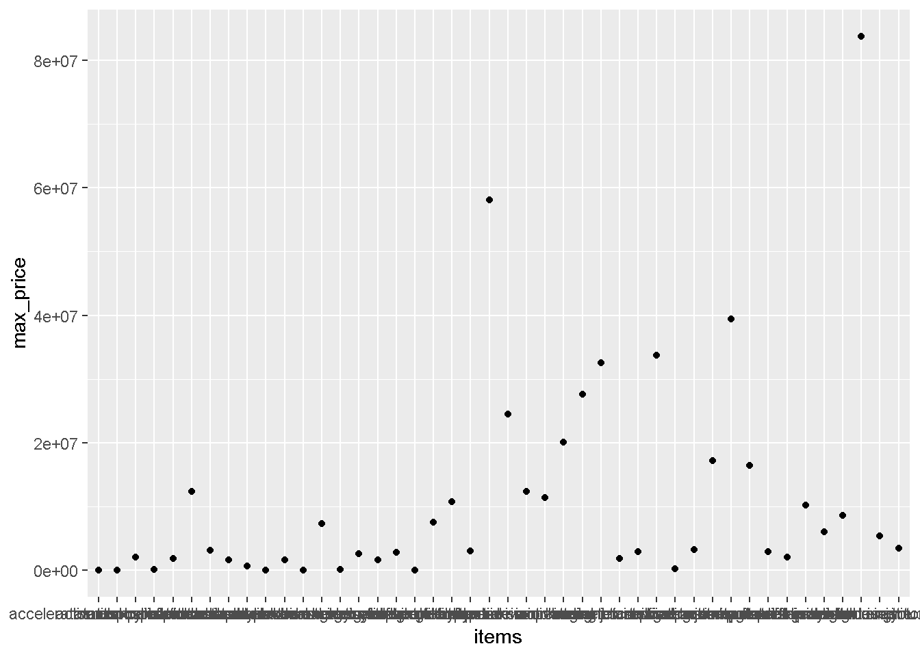
Try
coord_flip()to make the plot more readable. If you’re interested in learning more aboutcoord_flip(), ask R for help!?coord_flip
Show solution
ggplot(data = summary_scrap, aes(items, max_price)) +
  geom_col() +
  coord_flip()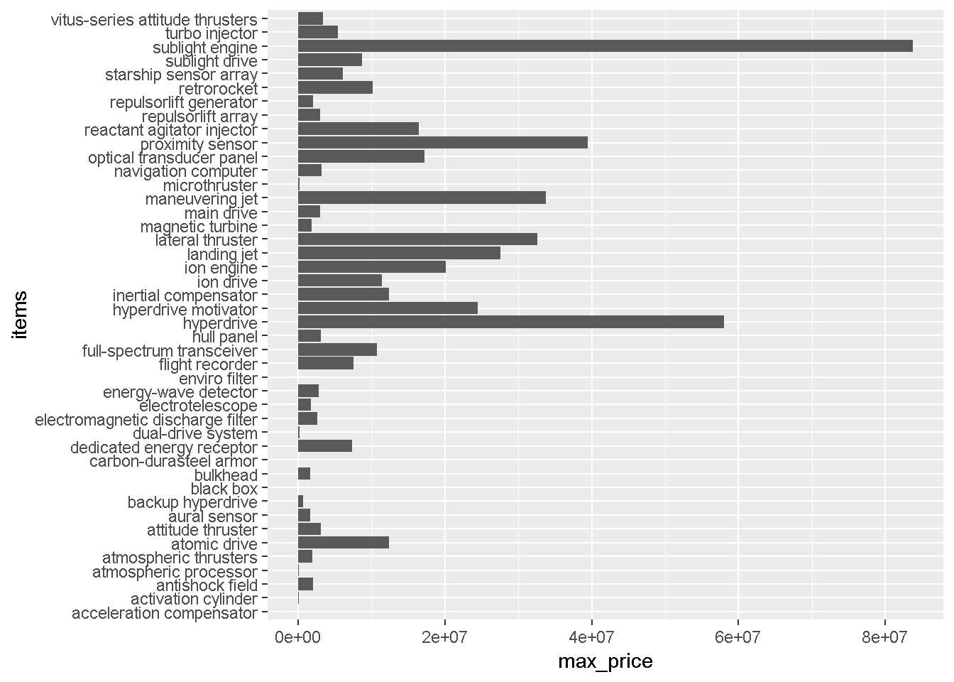
This plot might look a lot better if the maximum data were sorted. Try reorder() to make this chart way more readable. Type “?reorder” to learn more about that function.
Show solution
ggplot(data = summary_scrap, aes(reorder(items, max_price), max_price)) +
  geom_col() +
  coord_flip()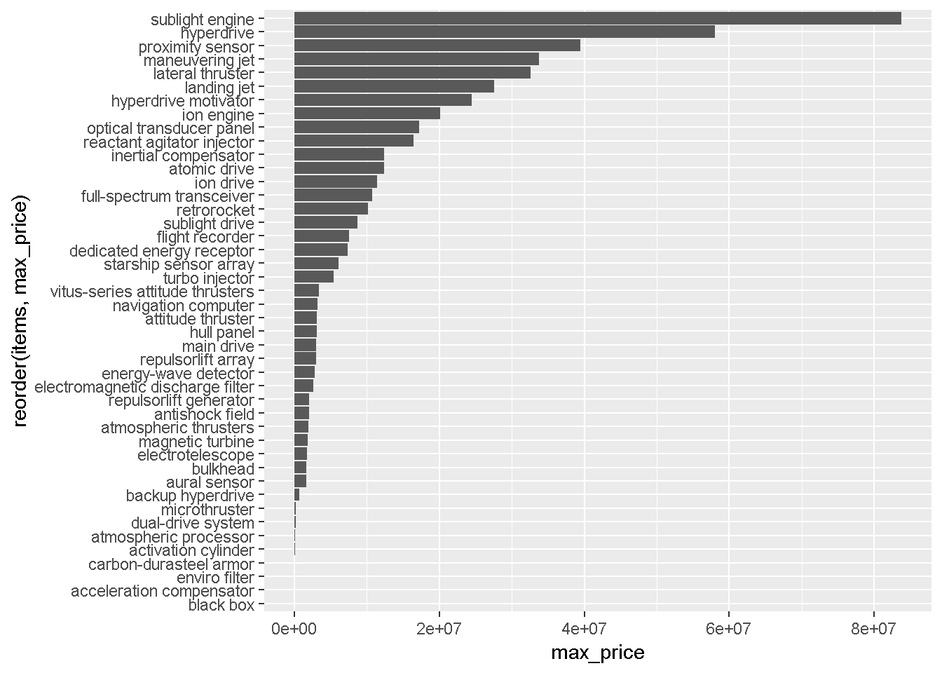
Nice work!! You may now move on to the Commodore level analysis.